📖 Multiplicity of Equilibria in Static Games

⏱ | words

Practical task 7.1 Practical task 7.2 Practical task 7.3 References

Simple static game of incomplete information with multiple equilibria

Main paper:

📖 Su [2014] “Estimating discrete-choice games of incomplete information: Simple static examples”

✝︎ Che-Lin Su, 1974-2015, Associate Professor of Operations Management at the University of Chicago Booth School of Business

Today:

• Investigation into multiplicity of equilibria using a simple example

• Practical implementation of a solver for multiple equilibria

Example: static entry game

• Two firms: \(a\) and \(b\)

• Actions: each firm has two possible actions:

\[\begin{split} d_a= \begin{cases} 1, & \text{if firm } a \text{ chooses to enter the market}\\ 0, & \text{if firm } a \text{ chooses not to enter the market} \end{cases} \end{split}\]

\[\begin{split} d_b= \begin{cases} 1, & \text{if firm } b \text{ chooses to enter the market}\\ 0, & \text{if firm } b \text{ chooses not to enter the market} \end{cases} \end{split}\]

• Simultanenous entry decisions in the beginning \(\impliedby\) static game

• Utility = payoffs to the firms

\[\begin{split} u_a(d_a, d_b, x_a, \varepsilon_a)= \begin{cases} [\alpha + d_b(\beta-\alpha)]x_{a} + \varepsilon_{a1}, & d_a=1\\ 0 + \varepsilon_{a0}, & d_a=0 \end{cases} \end{split}\]

\[\begin{split} u_b(d_a, d_b, x_b, \varepsilon_b)= \begin{cases} [\alpha + d_a(\beta-\alpha)]x_{b} + \varepsilon_{b1}, & d_b=1\\ 0 + \varepsilon_{b0}, & d_b=0 \end{cases} \end{split}\]

• \(x=(x_a, x_b)\): firms’ observed types, common knowledge

• \(\theta=(\alpha, \beta)\): structural parameters to be estimated

• \(\varepsilon = (\varepsilon_a,\varepsilon_b)=(\varepsilon_{a0},\varepsilon_{a1},\varepsilon_{b0},\varepsilon_{b1})\): firms’ unobserved types, private information

• \(\varepsilon\) are observed only by each firm, not by the opponent nor the econometrician \(\implies\) game of incomplete information \(\implies\) Bayesian Nash equilibrium (BNE), CCPs in focus of the solution method

• Let beliefs of the other firm’s action be given by \(p_a = Pr\{d_a =1\}\), \(p_b = Pr\{d_b =1\}\) \(\iff\) CCPs in the equilibrium will be given by \(p^*_a\) and \(p^*_b\), with beliefs consistent with behavior

• Expected (with respect to beliefs about the other player) profits are

\[\begin{split} \mathbb{E}u_a(d_a, d_b, x_a, \varepsilon_a)= \begin{cases} [\alpha + p_b(\beta-\alpha)]x_{a} + \varepsilon_{a1}, & d_a=1\\ 0 + \varepsilon_{a0}, & d_a=0 \end{cases} \end{split}\]

\[\begin{split} \mathbb{E} u_b(d_a, d_b, x_b, \varepsilon_b)= \begin{cases} [\alpha + p_a(\beta-\alpha)]x_{b} + \varepsilon_{b1}, & d_b=1\\ 0 + \varepsilon_{b0}, & d_b=0 \end{cases} \end{split}\]

• Assume the error terms \((\varepsilon_{a0},\varepsilon_{a1},\varepsilon_{b0},\varepsilon_{b1})\) are iid across firms and alternatives, centralized and normalized EV1 distribution

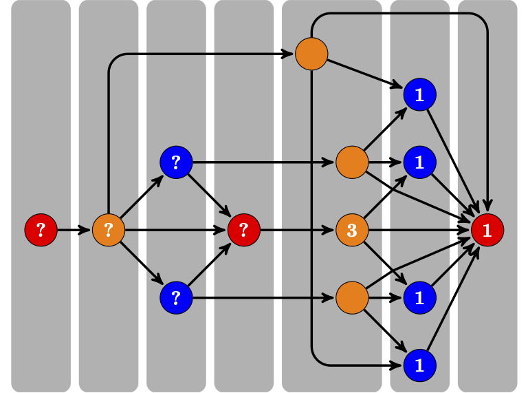
• Choice probabilities are then given by

\[ p_{a}= \frac{\exp[p_{b}\beta x_{a} +(1-p_{b})\alpha x_{a}] }{1+\exp[p_{b}\beta x_{a} +(1-p_{b})\alpha x_{a}]} = \frac{1}{1+\exp[-\alpha x_{a} + p_{b}x_{a}(\alpha-\beta)]} \equiv \Psi_{a}(p_b,x,\theta) \]

\[ p_{b}= \frac{\exp[p_{a}\beta x_{b} +(1-p_{a})\alpha x_{b}] }{1+\exp[p_{a}\beta x_{b} +(1-p_{a})\alpha x_{b}]} = \frac{1}{1+\exp[-\alpha x_{b} + p_{a}x_{b}(\alpha-\beta)]} \equiv \Psi_{b}(p_a,x,\theta) \]

• Define the equilibrium mapping

\[ \Psi: [0,1]^2 \ni (p_a,p_b) \mapsto (p_a,p_b) \in [0,1]^2 \]

\[ \Psi(p_a,p_b) = \big[\Psi_{a}(p_b,x,\theta), \Psi_{b}(p_a,x,\theta)\big] \]

Definition

A Bayesian-Nash equilibrium is given by a pair of CCPs of the players which constitutes mutual best responses to each others’ strategies. Thus, the equilibrium CCPs given by \((p^*_a,p^*_b)\) satisfy the fixed point equation

\[ (p^*_a,p^*_b) = \Psi(p^*_a,p^*_b). \]

Existence of BNE? Multiplicity of BNE?

Solving for equilibria

Parameterization

We consider a very contestable game throughout:

• Monopoly profits: \(\alpha x_{j}=5x_{j}\)

• Duopoly profits: \(\beta x_{j}=-11x_{j}\)

• Firm types: \((x_a ,x_b) = (0.52, 0.22)\)

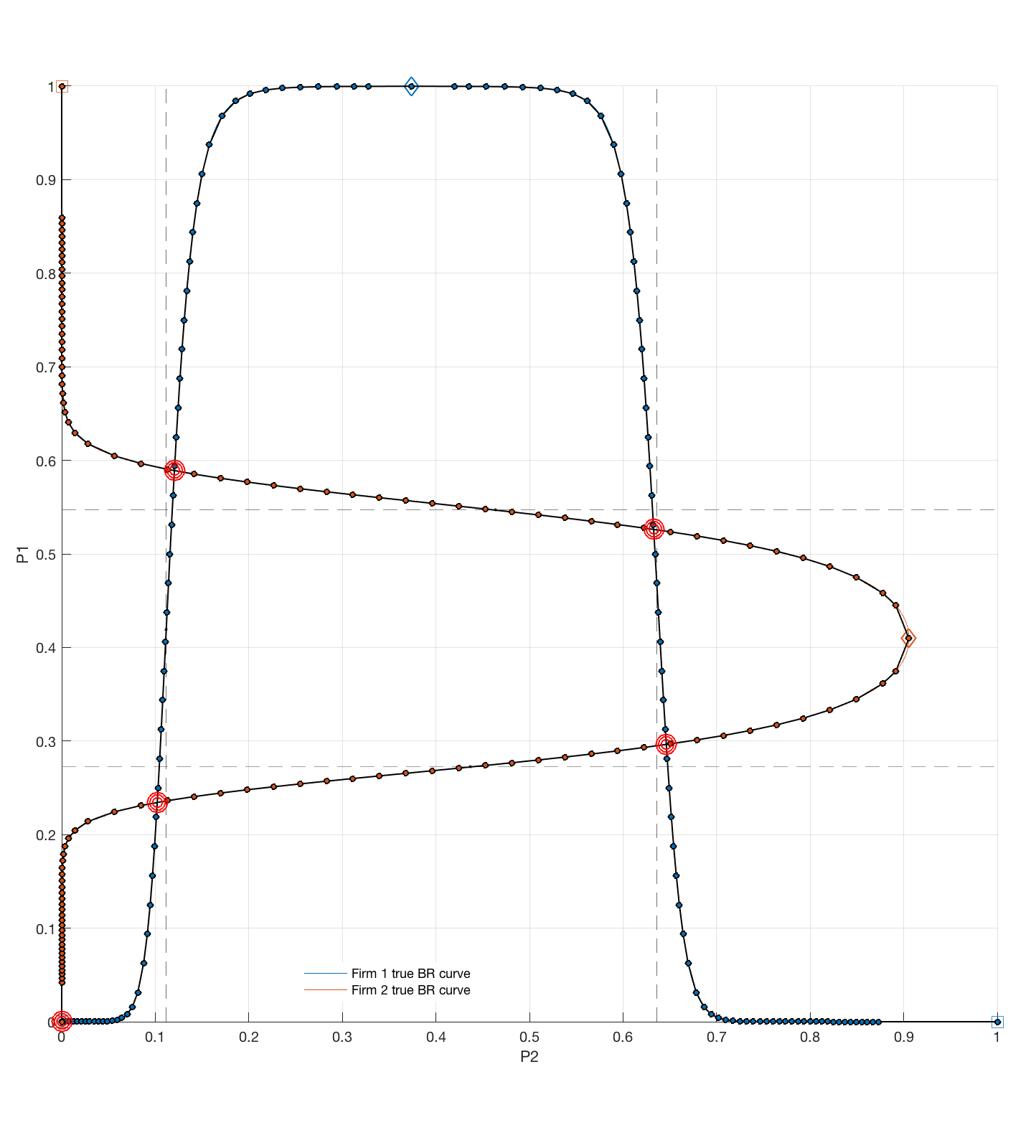
Solution approach 1

• equilibria are intersections of best response functions

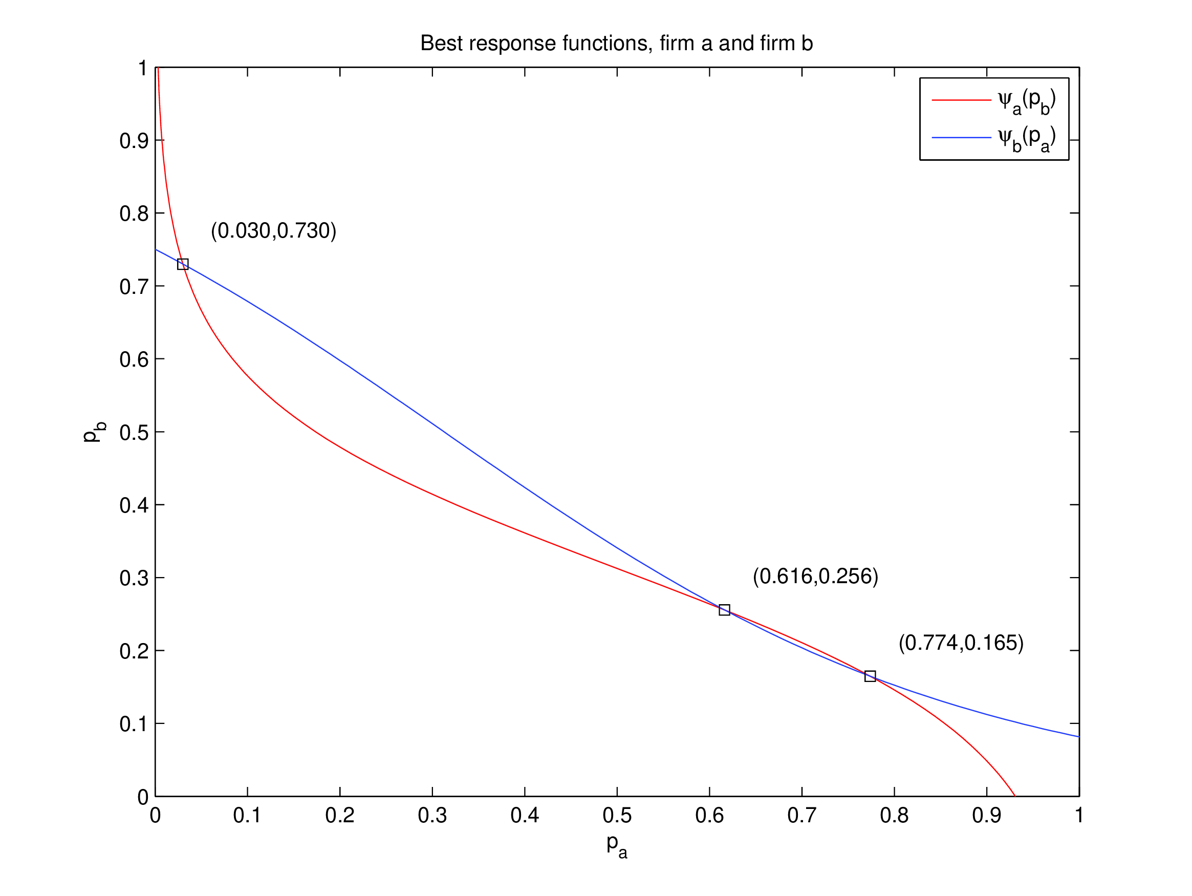
Three equilibria!!!

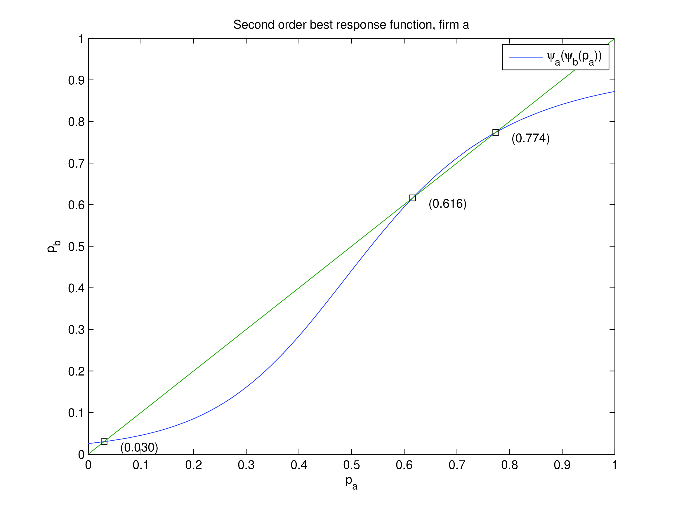
Solution approach 2

• equilibria as fixed point of second-order best response function

• Second-order best response function

\[ \psi_a\big(\psi_b(p_a)\big): p_a \mapsto p_a \]

How to solve to find all equilibria?

• No absolutely guaranteed method to find all equilibria

• Poly-algorithm is a good idea

• Approximation is a good idea

• Adaptive update of the solution to increase accuracy is a good idea

Combination of successive approximations and the bisection algorithm.

1. Successive approximations (SA)

• Converges to the nearest stable equilibrium.

• Start SA at \(p_{a}=0\) and \(p_{a}=1\).

• Unique equilibrium (\(K=1\)): SA converges from anywhere.

• Three equilibria (\(K=3\)): two stable, one unstable.

• More equilibria (\(K>3\)): not in this model.

2. Bisection method

• Use to find the unstable equilibrium when \(K=3\).

• Repeatedly bisect an interval and select the subinterval where the fixed point/root lies.

• The two stable equilibria define the initial search interval.

• Very simple and robust, but relatively slow.

Piecewise linear approximations

• simple idea of approximating best response curves by piecewise linear functions

• how many segments?

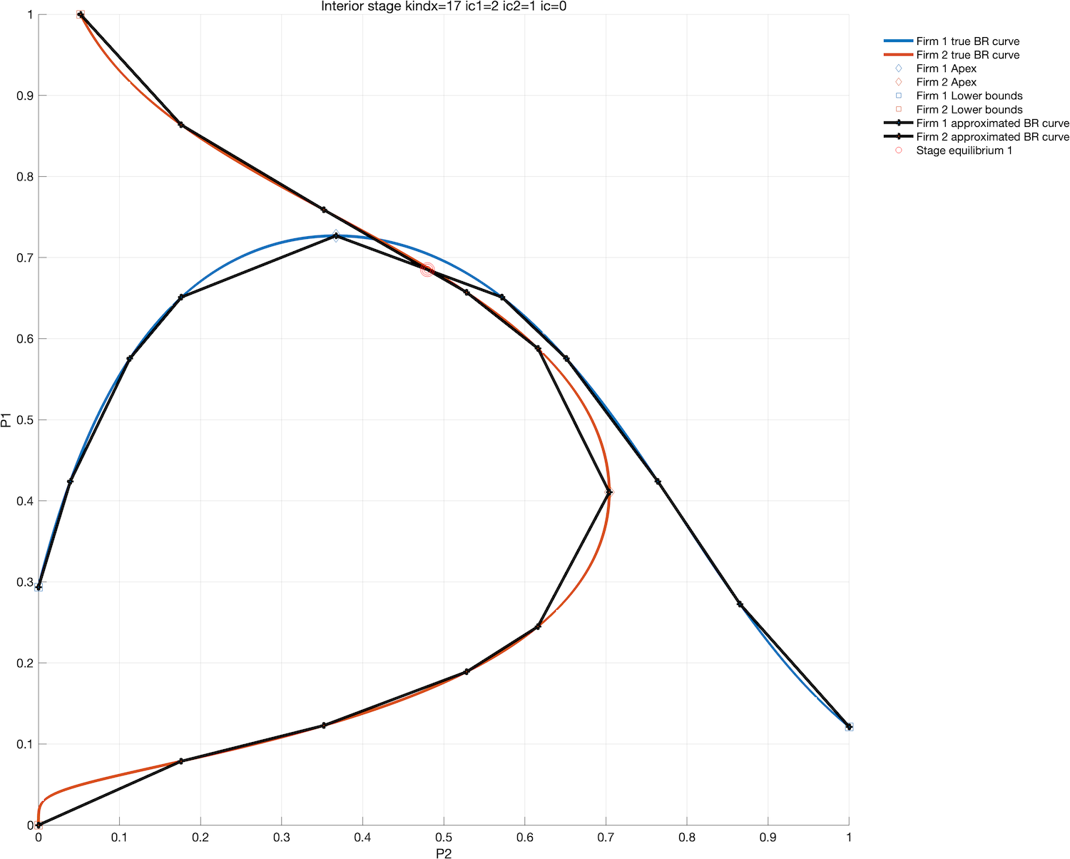
• adoptive procedure is always a good idea!

• make a sequential refinement procedure

• the difference between current and previous step gives a measure of the approximation error

• perform another step until the error is smaller than preset tolerance level

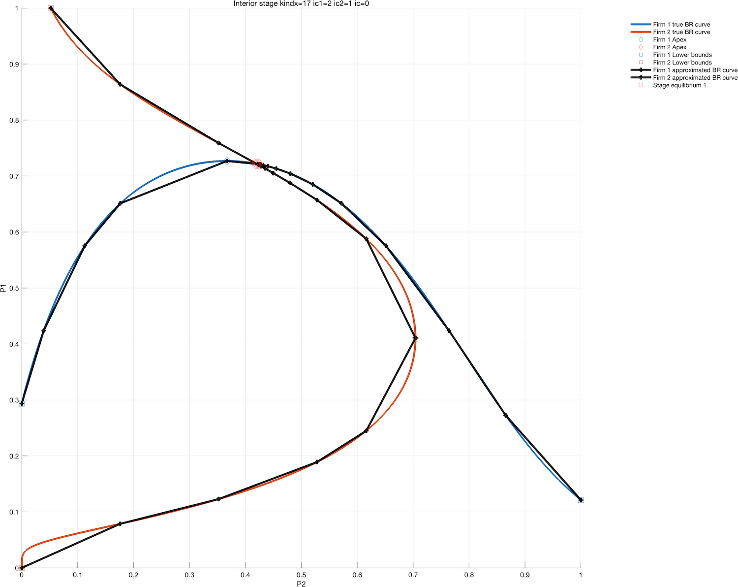
• can handle arbitrary complex best response functions

• any number of regular equilibria

• numerical stability issues when best responses close to 0 or 1, which happens often

Practical Task 7.1

• Study the implementing Su(2014) static model

• Play with the model

• Test the limits of the fixed point solver

Find the exercise code and materials in the exercises repo in the forlder 7_multiplicity

Practical Task 7.2

• Study the implementation of piecewise linear approximations in class polyline

• Watch the development of polyline class in a video from my CompEcon course

• Code up a solver based on polylines, with adaptive refinement [optional]

• Compare the accuracy of the solution to the fixed point solver

Find the exercise code and materials in the exercises repo in the forlder 7_multiplicity

Structural Estimation

• Data Generating Process (DGP): the data are generated by a single equilibrium

• The two players play the same equilibrium 1000 times

• Observed characteristics of the players are fixed at \((x_a ,x_b)=(0.52,0.22)\)

• Data: \(X=\{d_a^i ,d_b^i\}_{i=1}^{1000}\)

• True parameters: \(\theta=(\alpha_{0},\beta_{0})=(5,-11)\)

• Given data \(X\), we want to recover structural parameters \(\alpha\) and \(\beta\)

Static Game Example: Maximum Likelihood Estimation

• Maximize the likelihood function:

\[ \max_{\alpha,\beta}\ \log \mathcal{L}(p_{a}(\alpha,\beta);X) = \sum_{i=1}^{N}\!\left(d_{a}^i \log p_{a}(\alpha,\beta) + (1-d_{a}^i)\log[1-p_{a}(\alpha,\beta)]\right) \]

\[ + \sum_{i=1}^{N}\!\left(d_{b}^i \log p_{b}(\alpha,\beta) + (1-d_{b}^i)\log[1-p_{b}(\alpha,\beta)]\right). \]

• \(p_{a}(\alpha,\beta)\) and \(p_{b}(\alpha,\beta)\) solve the BNE equations:

\[ p_{a}= \frac{1}{1+\exp[-\alpha x_{a} + p_{b}x_{a}(\alpha-\beta)]} \equiv \Psi_{a}(p_{b},x_{a};\alpha,\beta), \]

\[ p_{b}= \frac{1}{1+\exp[-\alpha x_{b} + p_{a}x_{b}(\alpha-\beta)]} \equiv \Psi_{b}(p_{a},x_{b};\alpha,\beta). \]

MLE with nested full solution method (NFXP)

1. Outer loop

• Choose \((\alpha,\beta)\) to maximize the likelihood

\[ \log \mathcal{L}(p_{a}(\alpha,\beta),p_{b}(\alpha,\beta);X). \]

2. Inner loop

• For a given \((\alpha,\beta)\), solve the BNE equations for all equilibria:

\[ (p^{k}_{a}(\alpha,\beta),p^{k}_{b}(\alpha,\beta)), k=1,\dots,K \]

• Choose the equilibrium with the highest likelihood:

\[ k^{*}=\arg\max_{k=1,\dots,K}\ \log \mathcal{L}\big(p^{k}_{a}(\alpha,\beta),p^{k}_{b}(\alpha,\beta);X\big), \]

• and set

\[ (p_{a}(\alpha,\beta),p_{b}(\alpha,\beta))=(p^{k^{*}}_{a}(\alpha,\beta),p^{k^{*}}_{b}(\alpha,\beta)). \]

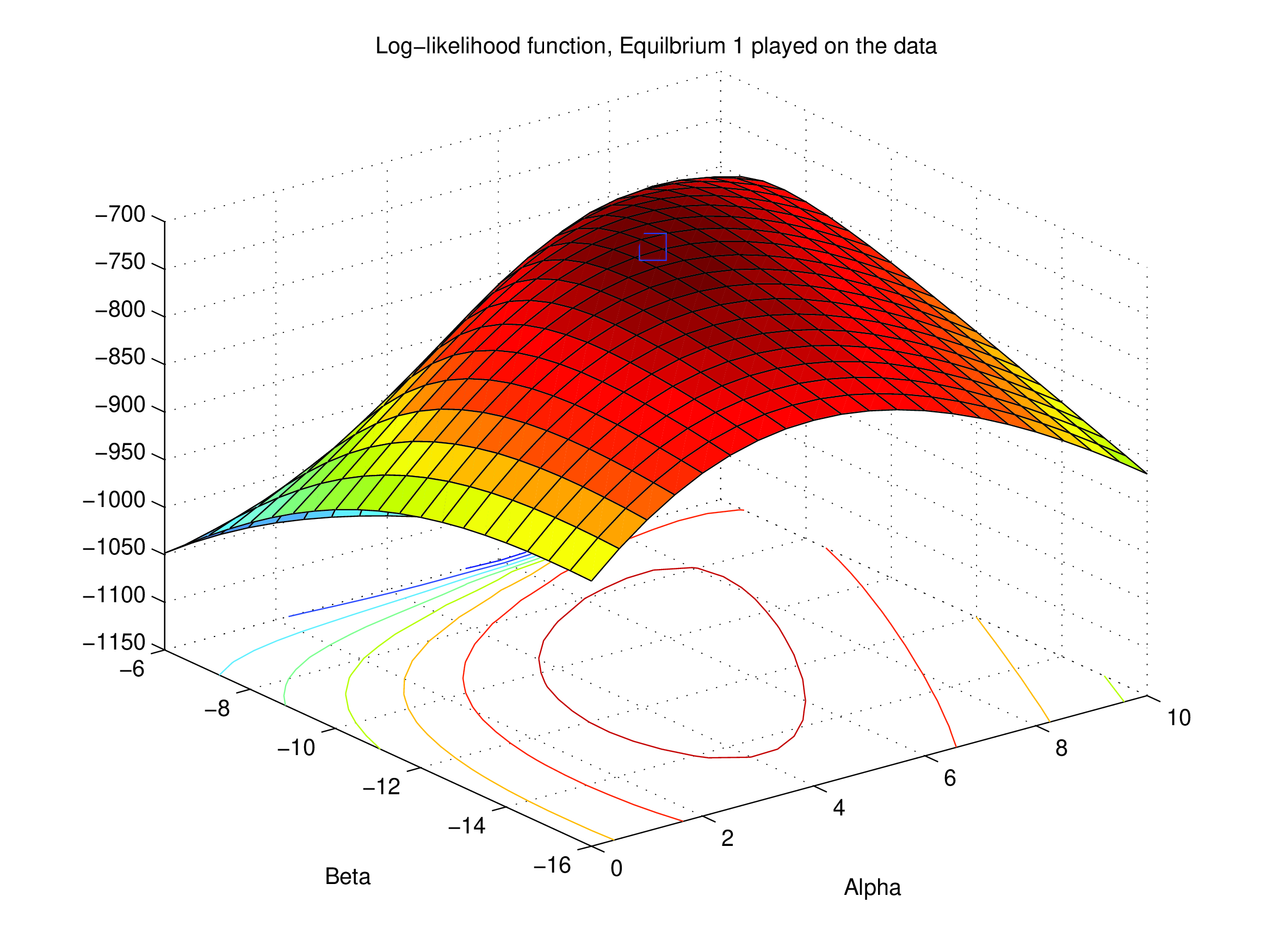
NFXP’s Likelihood as a Function of \((\alpha,\beta)\) — Eq 1

Data generated from equilibrium 1

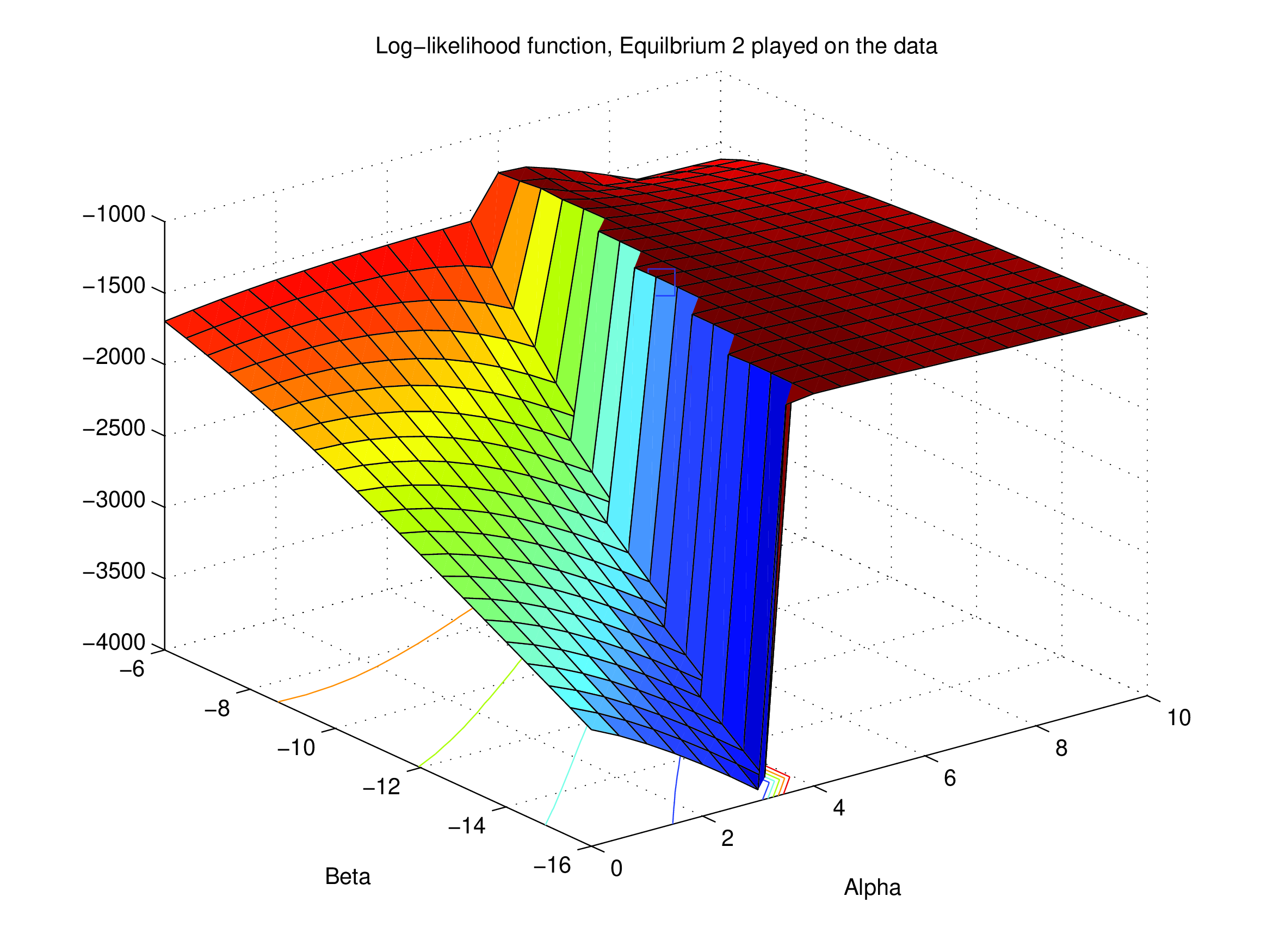
NFXP’s Likelihood as a Function of \((\alpha,\beta)\) — Eq 2

Data generated from equilibrium 2

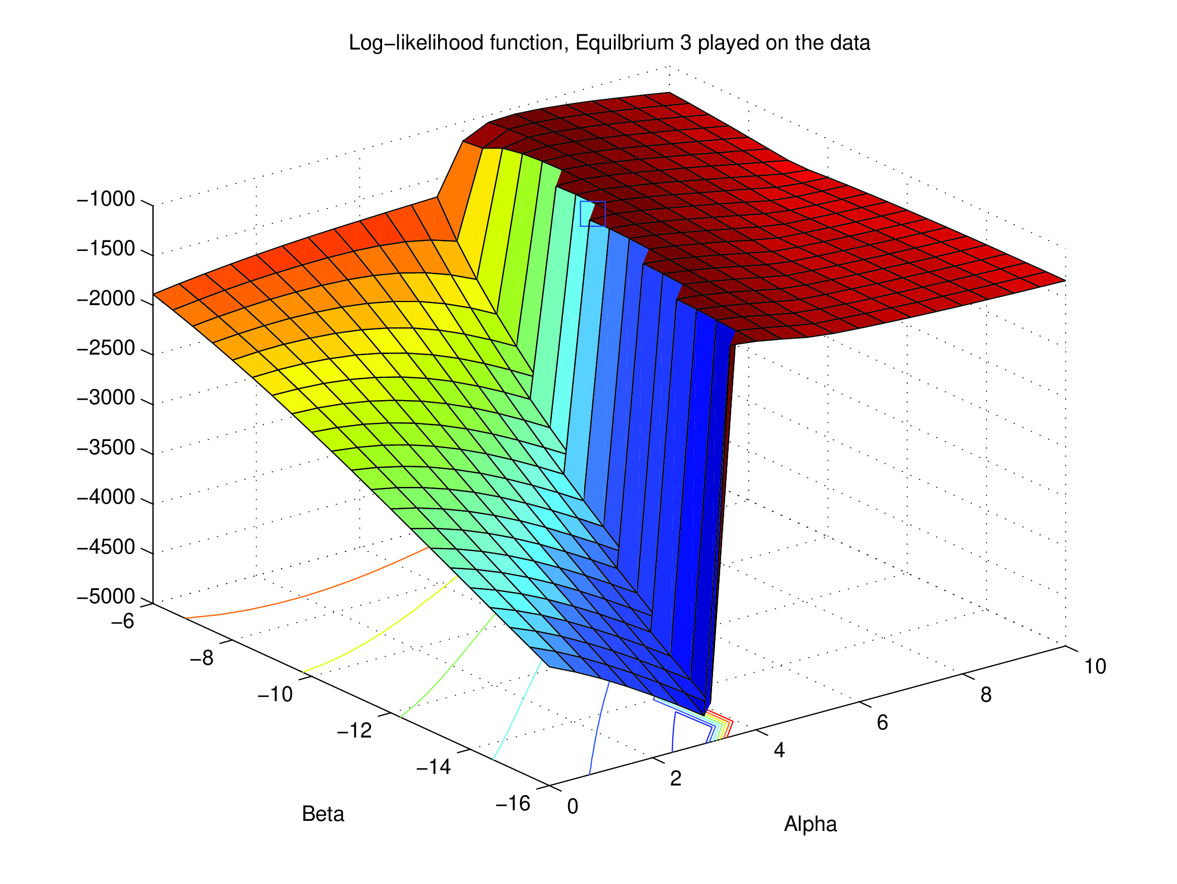
NFXP’s Likelihood as a Function of \((\alpha,\beta)\) — Eq 3

Data generated from equilibrium 3

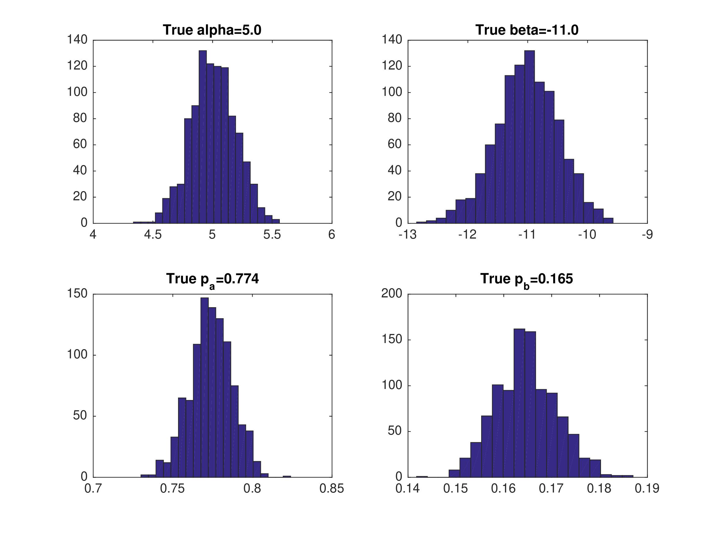
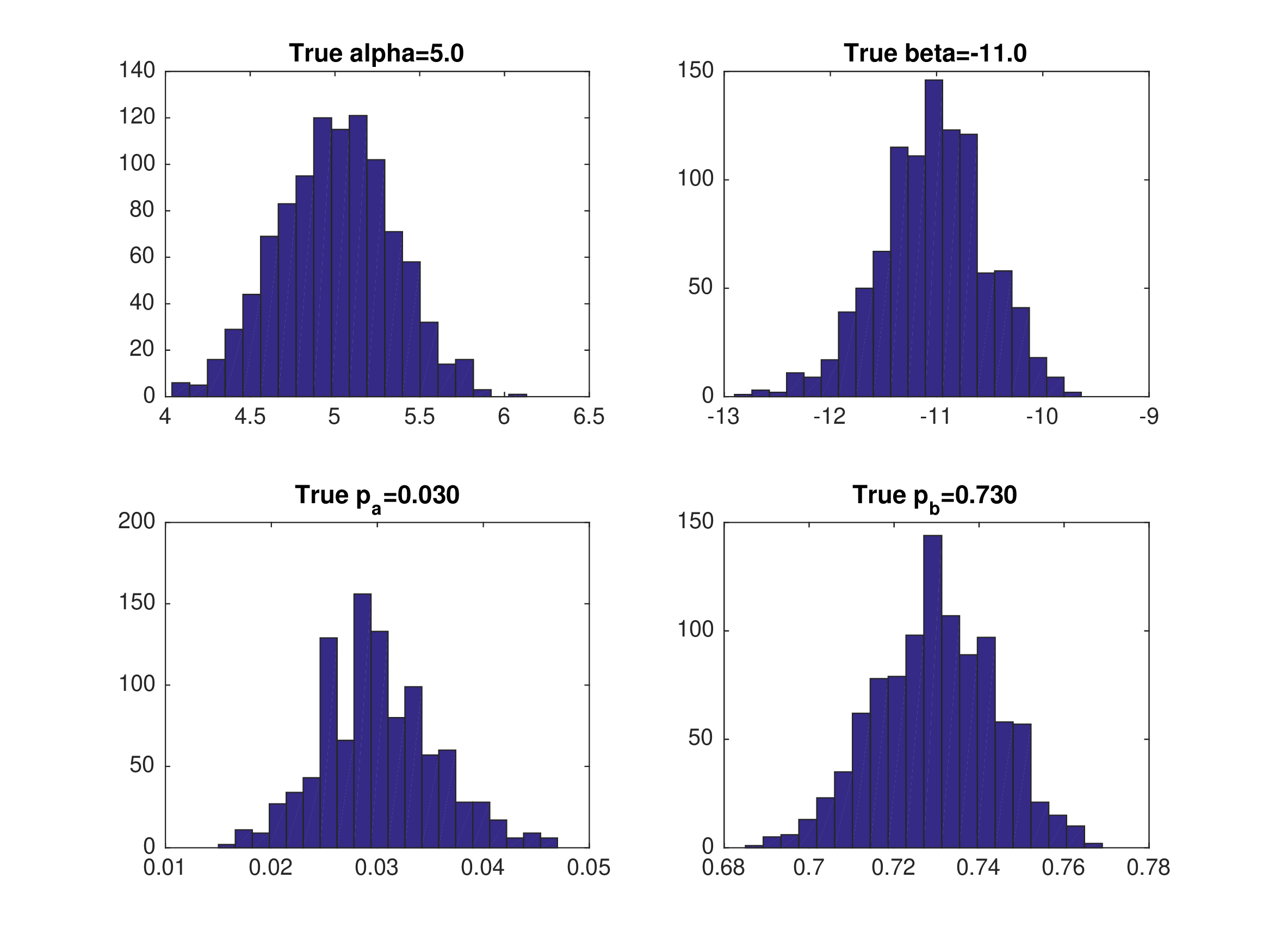
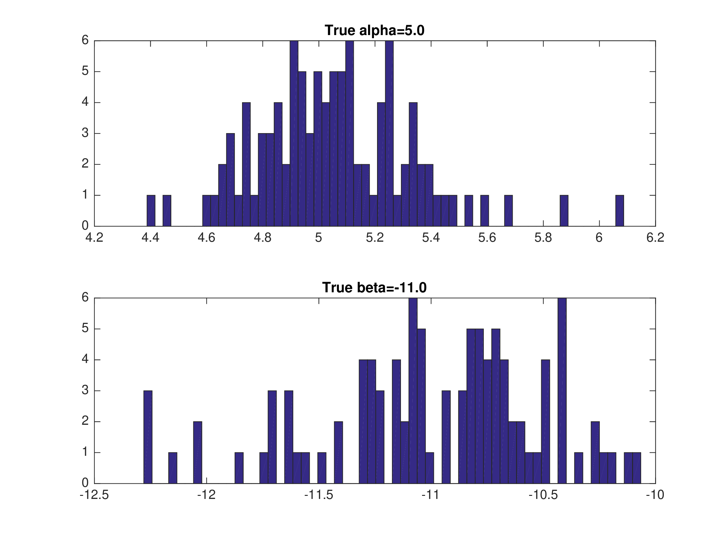
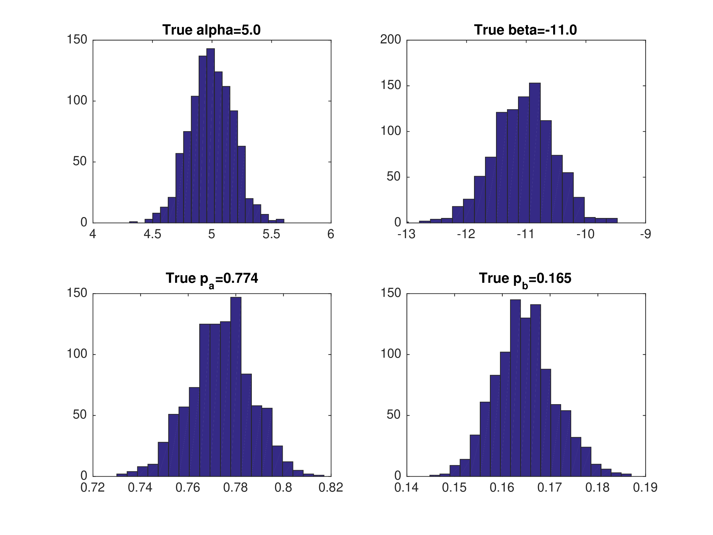
Monte Carlo Results: NFXP with Eq1

Data generated from equilibrium 1

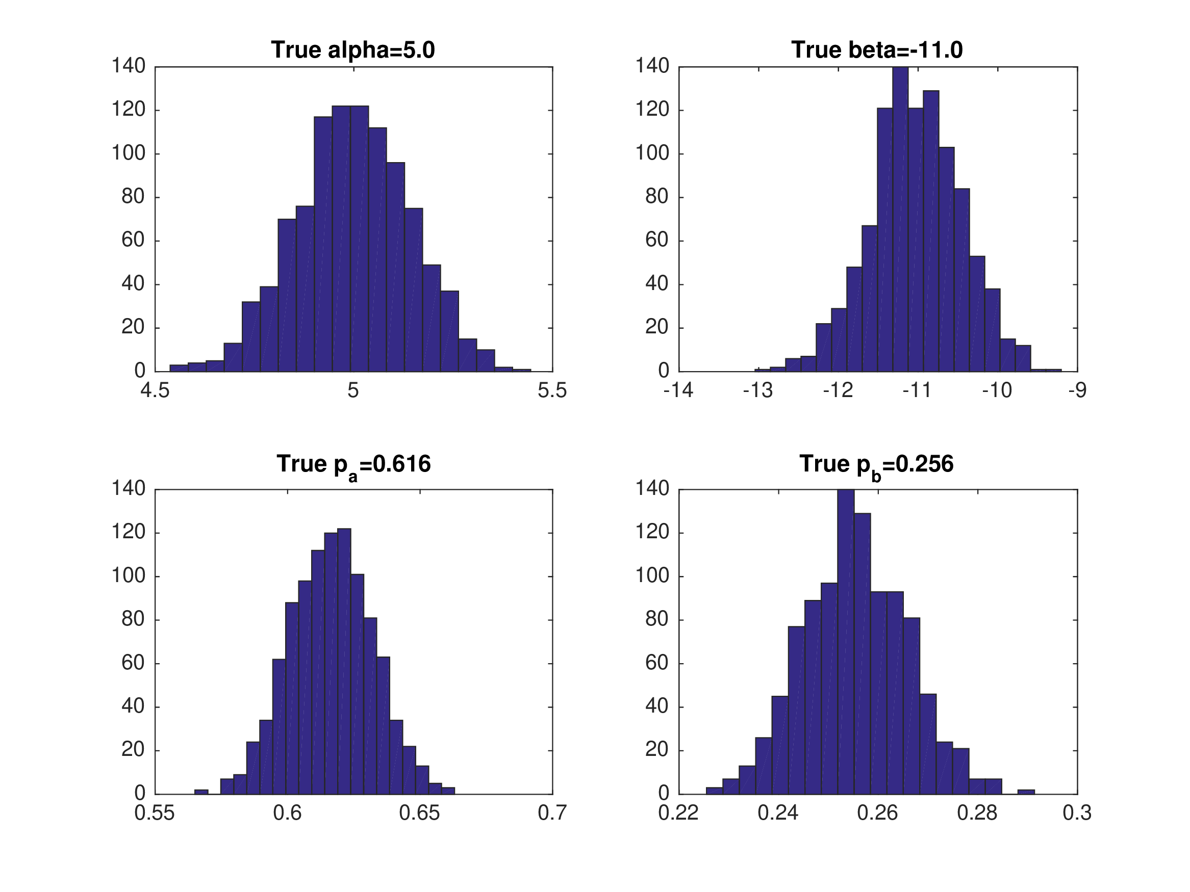
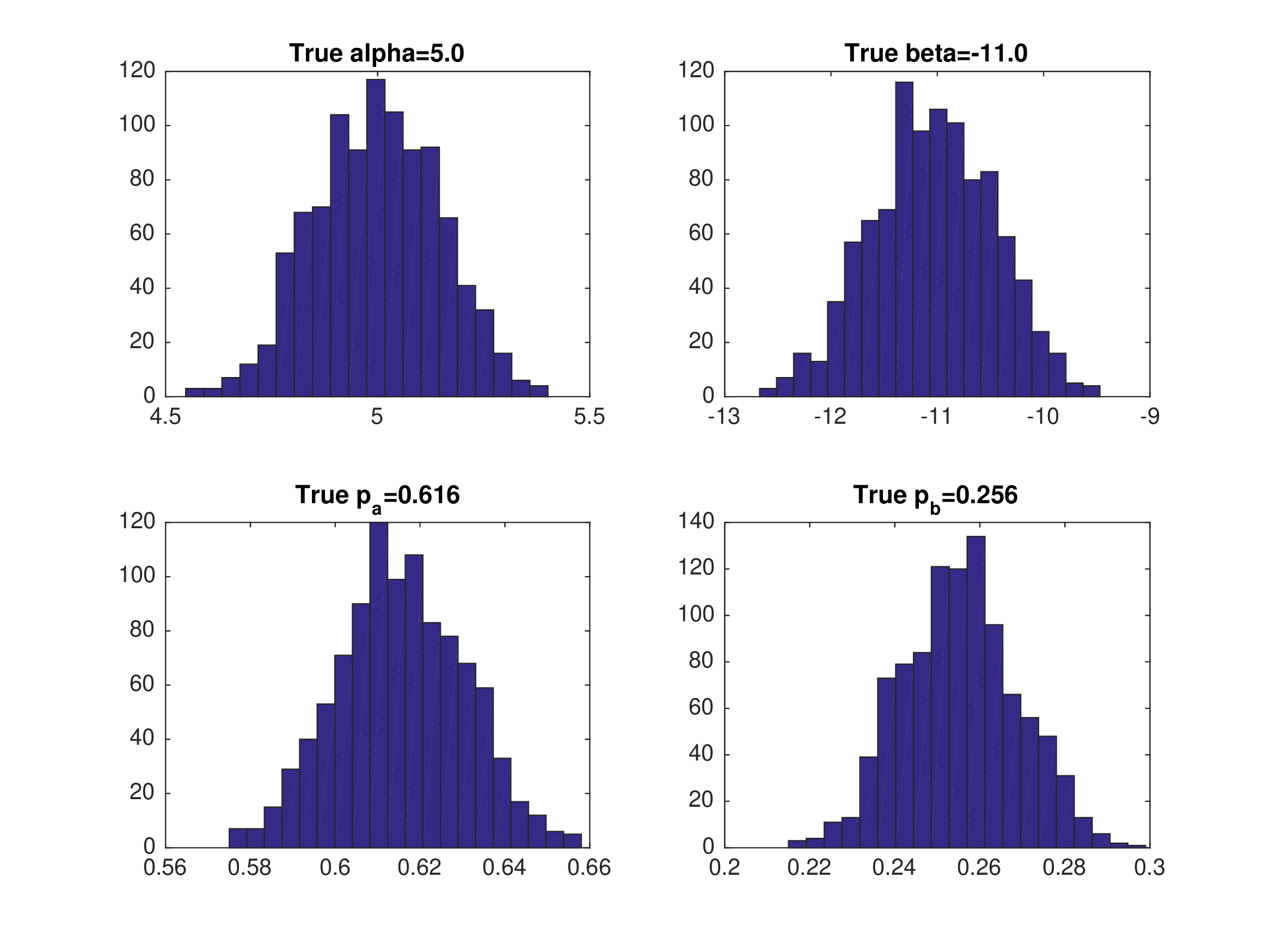
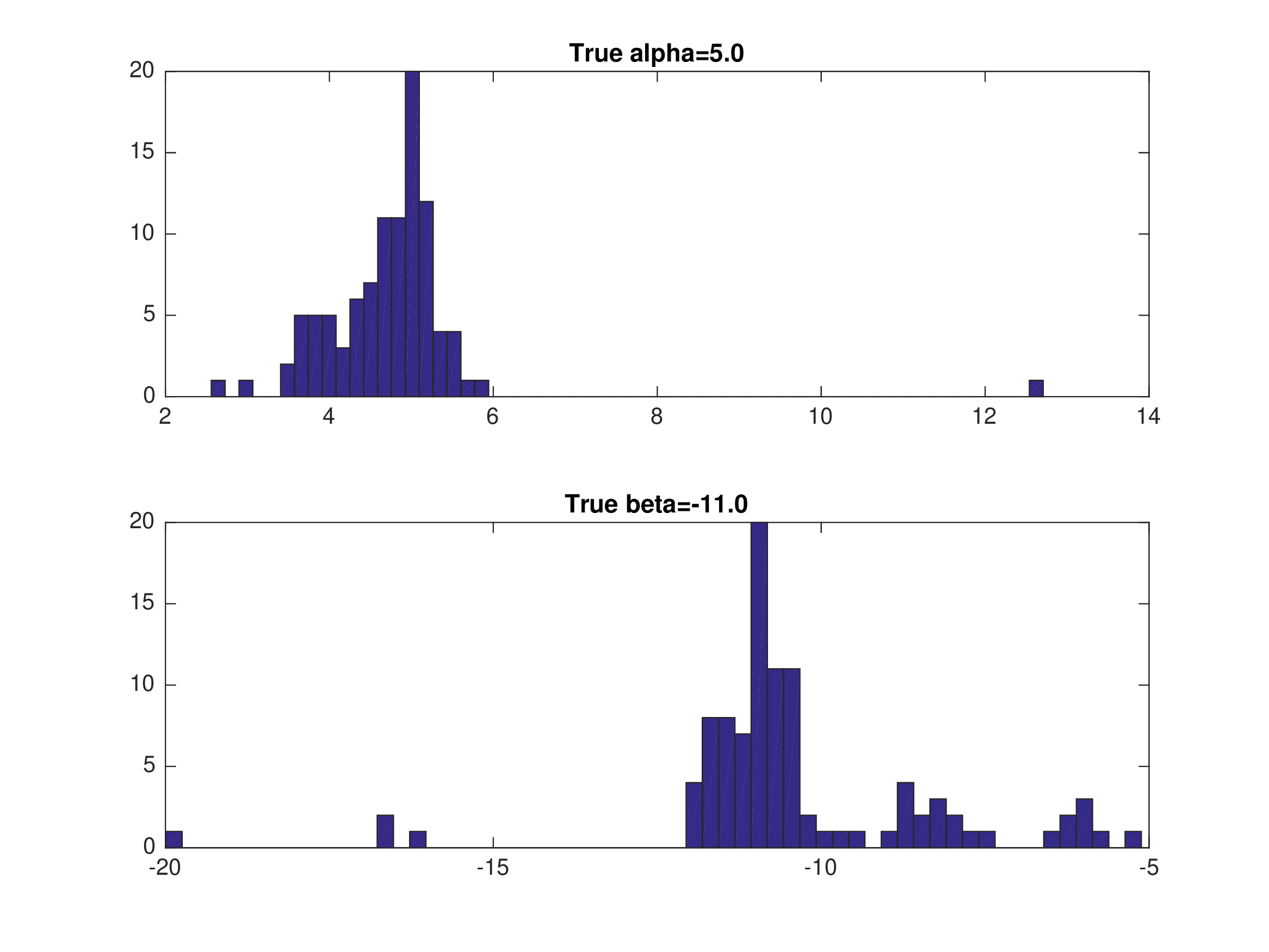
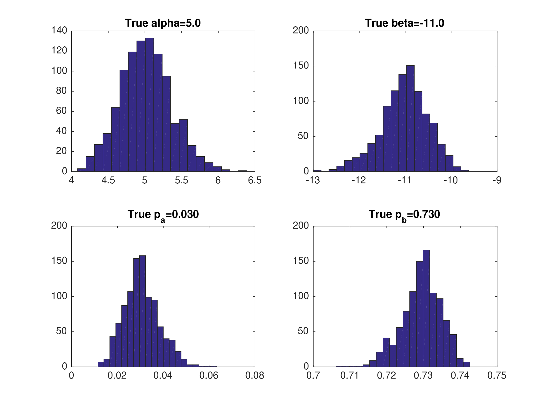
Monte Carlo Results: NFXP with Eq2

Data generated from equilibrium 2

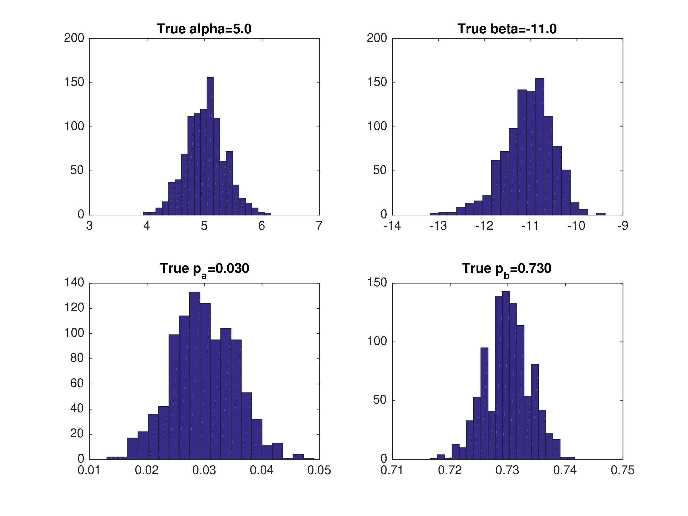
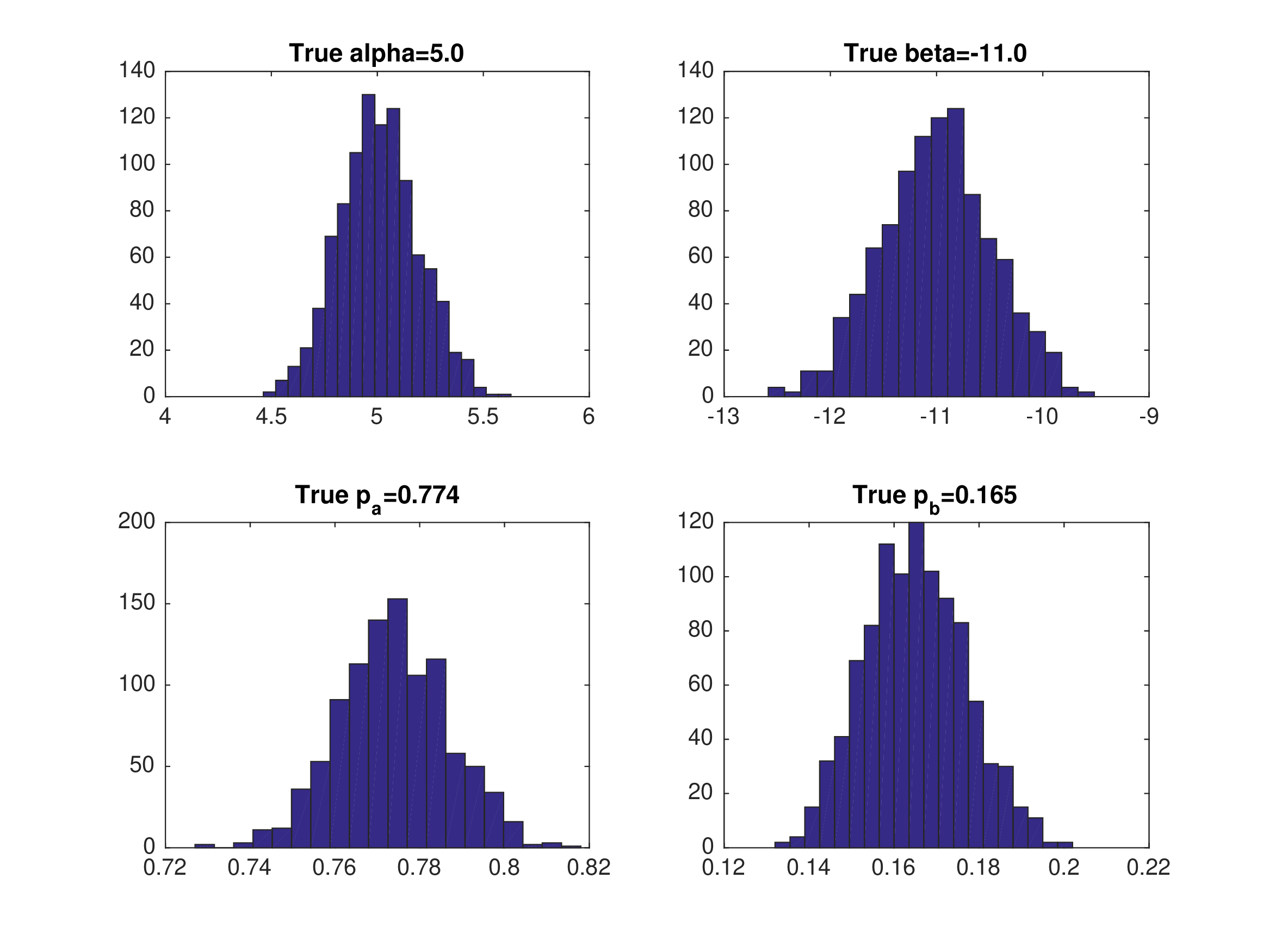
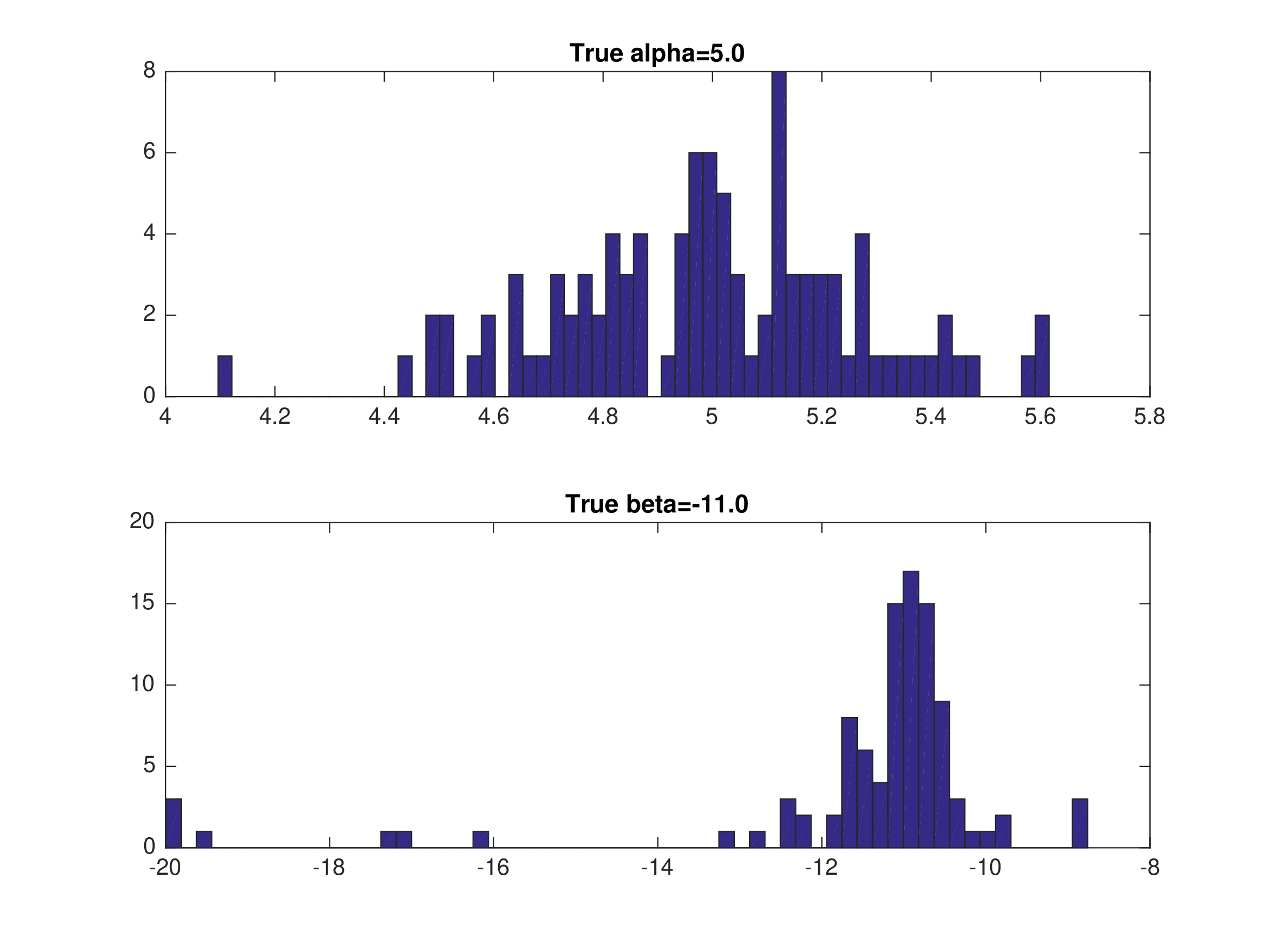
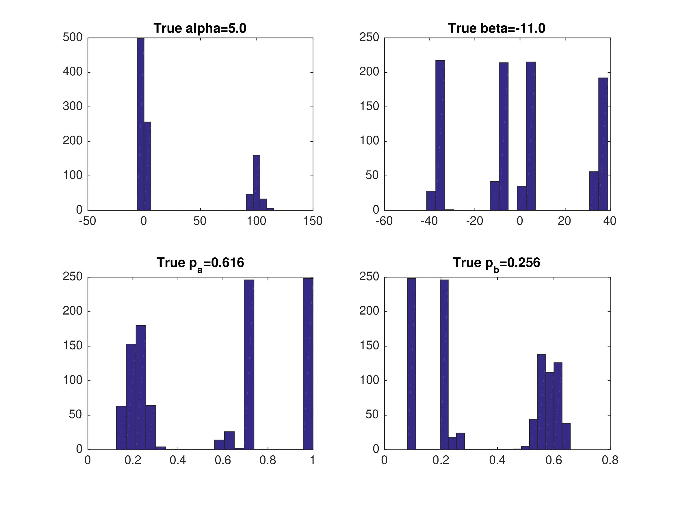
Monte Carlo Results: NFXP with Eq3

Data generated from equilibrium 3

Mathematical programming with equilibrium constraints (MPEC)

• Constrained Optimization Formulation for Maximum Likelihood Estimation

• Maximize the likelihood function:

\[ \max_{\alpha,\beta, p_{a}, p_{b}}\ \log \mathcal{L}(p_{a};X) = \sum_{i=1}^{N}\!\left(d_{a}^i \log p_{a} + (1-d_{a}^i)\log(1-p_{a})\right) + \sum_{i=1}^{N}\!\left(d_{b}^i \log p_{b} + (1-d_{b}^i)\log(1-p_{b})\right) \]

• Subject to BNE constraints:

\[ p_{a}= \frac{1}{1+\exp[-\alpha x_{a} + p_{b}x_{a}(\alpha-\beta)]},\qquad p_{b}= \frac{1}{1+\exp[-\alpha x_{b} + p_{a}x_{b}(\alpha-\beta)]}, \]

\[ 0\le p_{a},p_{b}\le 1. \]

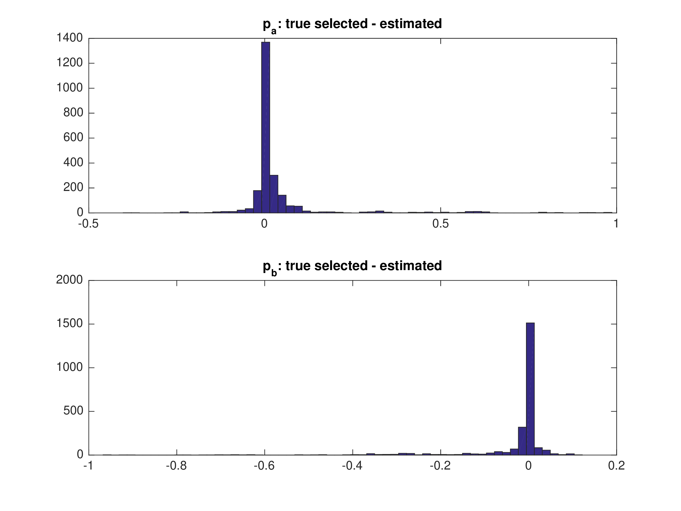
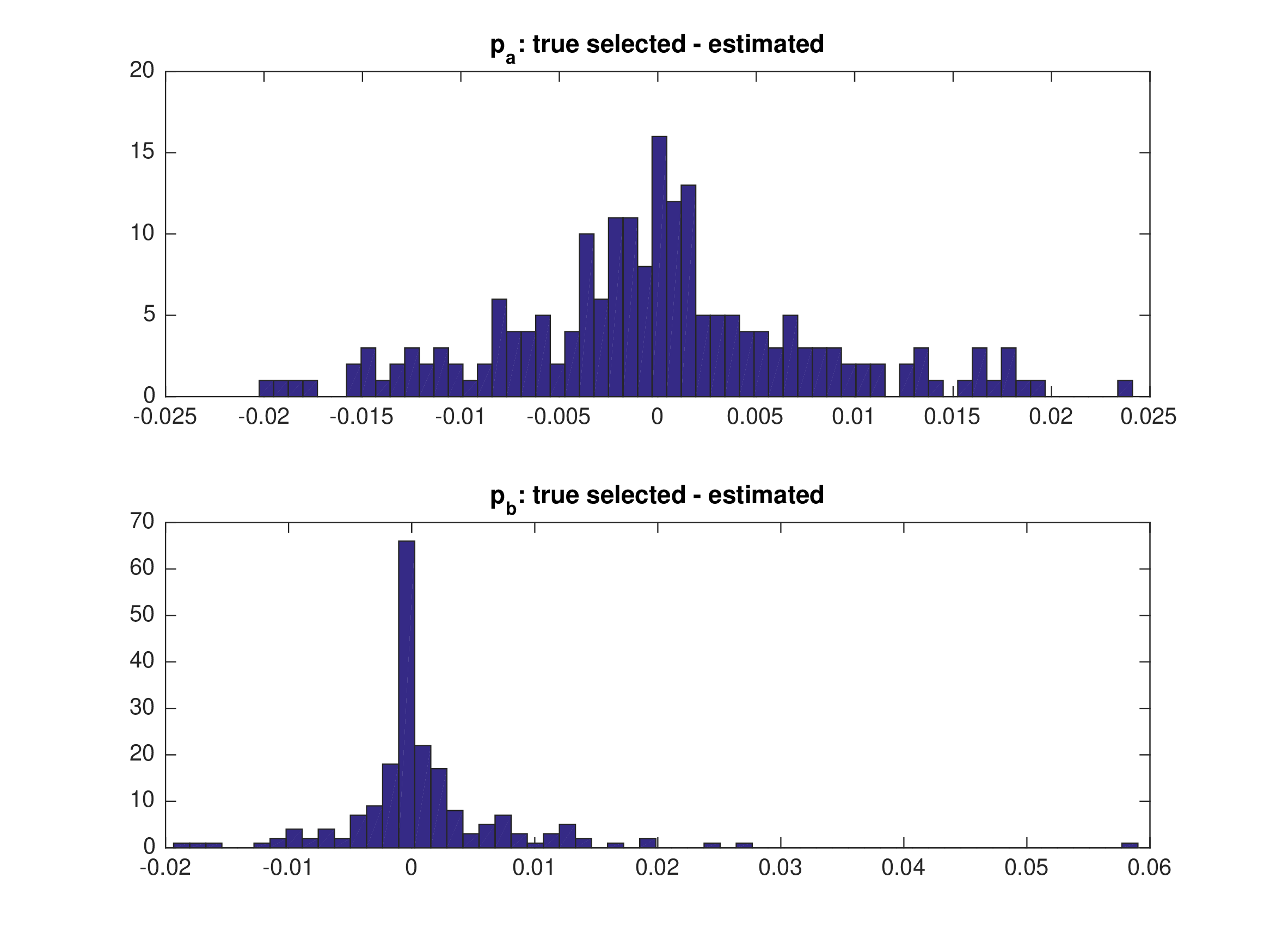
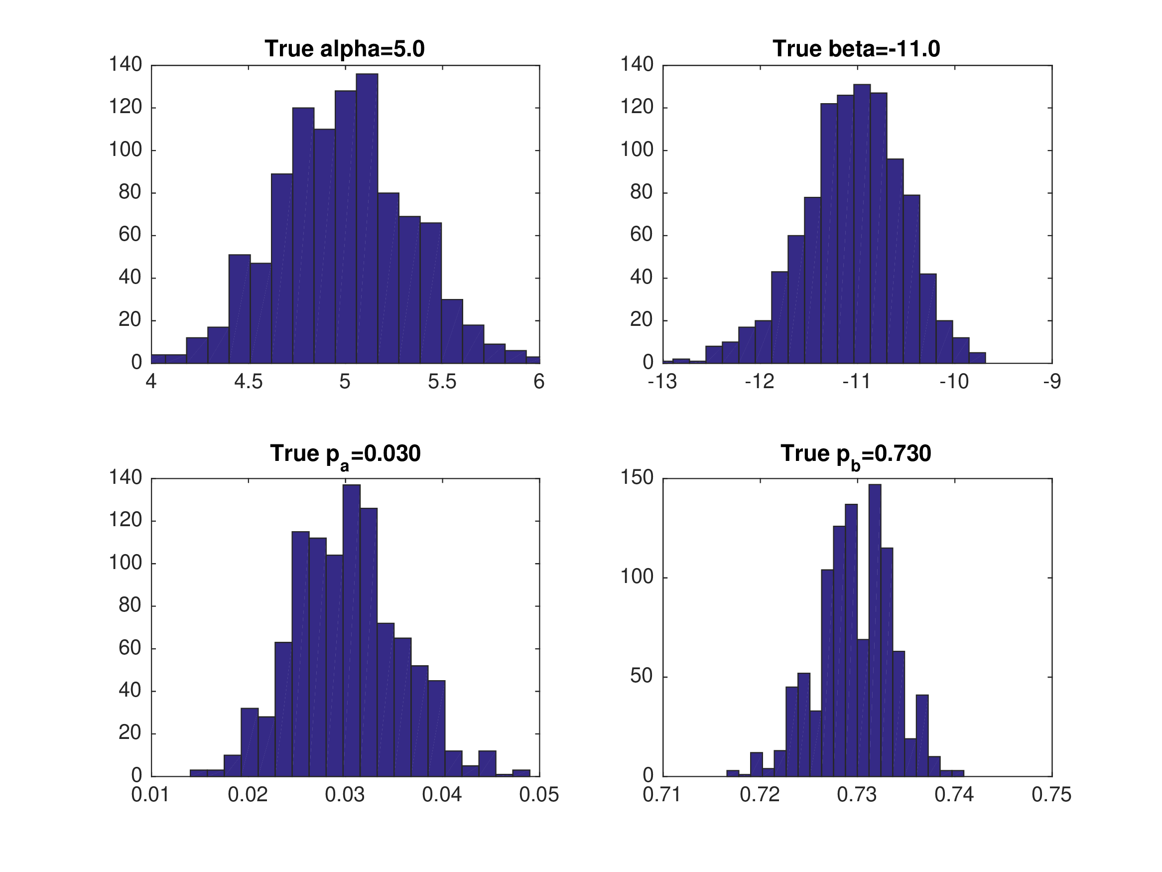
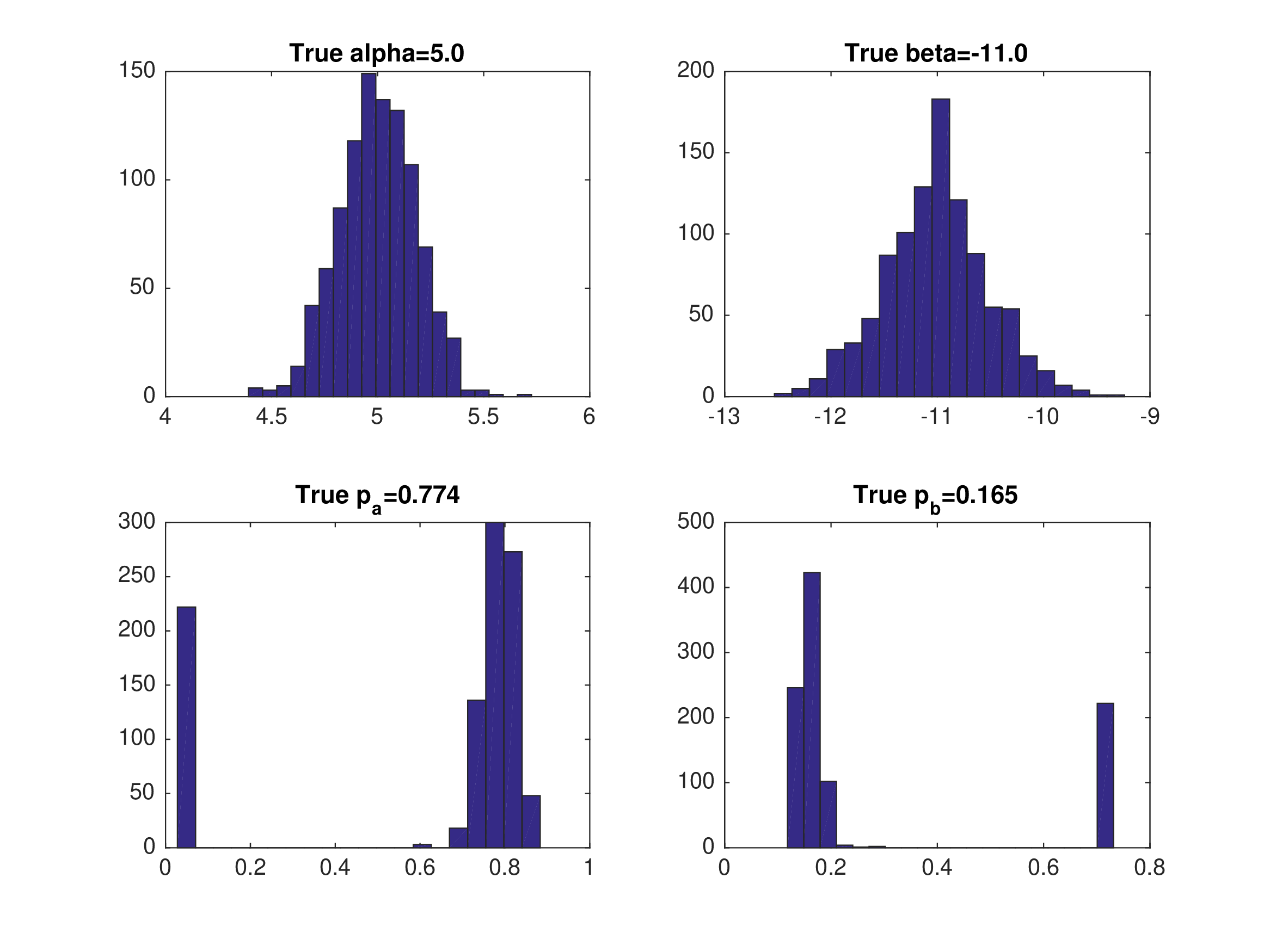
Monte Carlo Results: MPEC with Eq1

Data generated from equilibrium 1

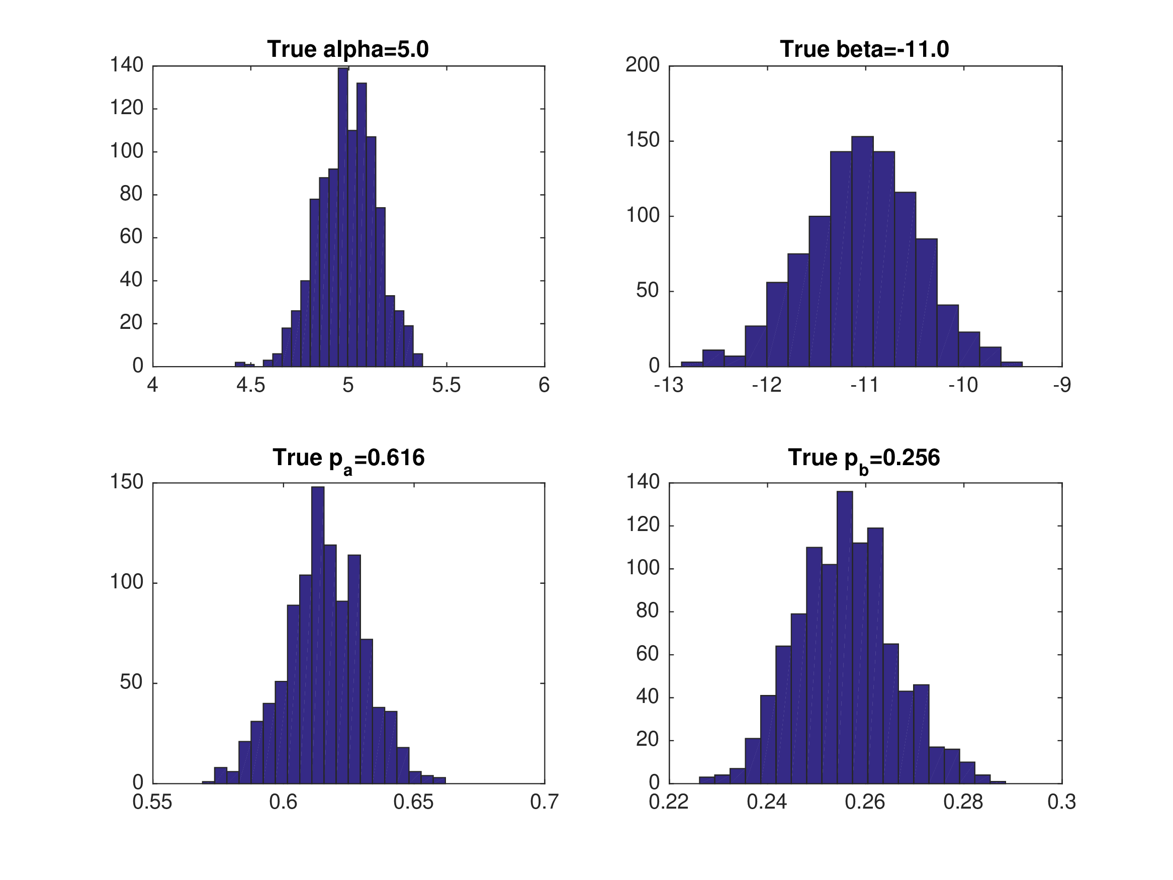
Monte Carlo Results: MPEC with Eq2

Data generated from equilibrium 2

Monte Carlo Results: MPEC with Eq3

Data generated from equilibrium 3

Static Game Example: Maximum Likelihood Estimation (repeat)

• Maximize the likelihood function (as above), with BNE definitions

\[ p_{a}= \frac{1}{1+\exp[-\alpha x_{a} + p_{b}x_{a}(\alpha-\beta)]} \equiv \Psi_{a}(p_{b},x_{a};\alpha,\beta), \]

\[ p_{b}= \frac{1}{1+\exp[-\alpha x_{b} + p_{a}x_{b}(\alpha-\beta)]} \equiv \Psi_{b}(p_{a},x_{b};\alpha,\beta). \]

Discussion

• Q: Is the likelihood function smooth in \(\alpha\) and \(\beta\) for NFXP? What about MPEC—are the objective and constraints smooth in \(\theta=(\alpha,\beta,p_a,p_b)\)?

• Q: Can we identify which equilibrium is played in the data (equilibrium selection rule)?

• Q: Can we use standard theorems for inference? Is the true value interior? Differentiable? Is the objective continuous?

• Q: This problem is extremely simple. \(p_a\) and \(p_b\) are scalars. How would you solve for \(p_a\) and \(p_b\) when they are solutions to players’ Bellman equations?

• Can we be sure to find all equilibria by iterating on players’ Bellman equations? Why/why not?

Estimation with Multiple Markets

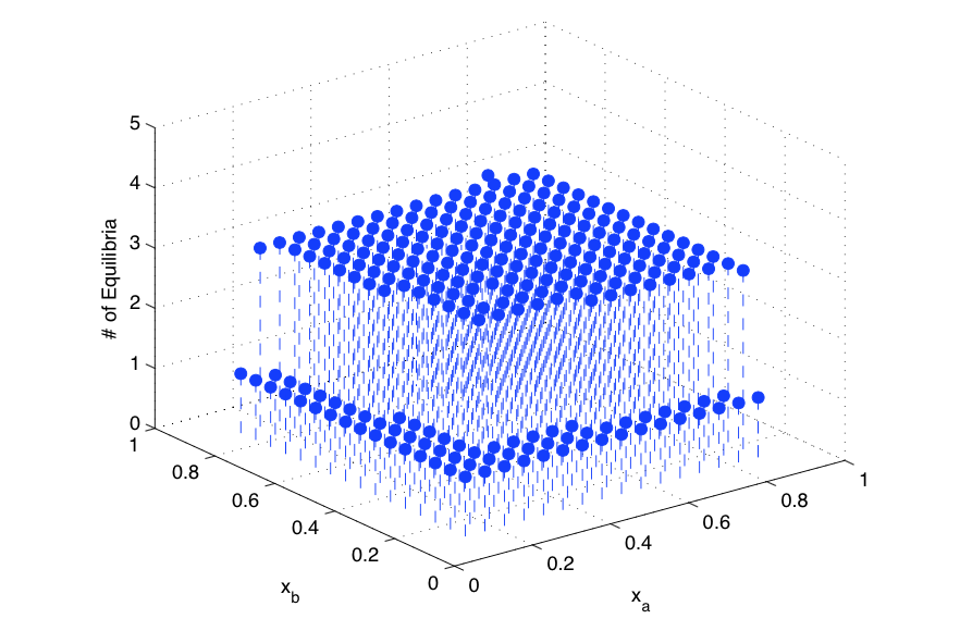
• There are 25 different markets, i.e. 25 pairs of observed types \((x^{m}_{a},x^{m}_{b})\), \(m=1,\dots,25\).

• The grid on \(x_a\) has 5 points equally distributed in \([0.12,0.87]\); similarly for \(x_b\).

• Use the same true parameter values \((\alpha_{0},\beta_{0})\).

• For each market \((x^{m}_{a},x^{m}_{b})\), solve BNE for \((p^{m}_{a},p^{m}_{b})\).

• There are multiple equilibria in most of the 25 markets.

• For each market, randomly choose an equilibrium to generate 1000 data points.

• The equilibrium used to generate data can differ across markets (randomized per market).

\(\implies\) # of Equilibria with Different \((x^{m}_{a},x^{m}_{b})\)

NFXP — Estimation with Multiple Markets

Inner loop:

\[ \max_{\alpha,\beta}\ \log \mathcal{L}\big(p^{m}_{a}(\alpha,\beta), p^{m}_{b}(\alpha,\beta);X\big). \]

Outer loop:

• For given \((\alpha,\beta)\), solve BNE for all equilibria \(k=1,\dots,K\) in each market \(m=1,\dots,M\):

\[ p^{m}_{a}= \Psi_{a}(p^{m}_{b},x^{m}_{a};\alpha,\beta),\qquad p^{m}_{b}=\Psi_{b}(p^{m}_{a},x^{m}_{b};\alpha,\beta). \]

• Choose, in each market, the equilibrium with the highest likelihood:

\[ k^{*}=\arg\max_{k=1,\dots,K}\ \log \mathcal{L}\big(p^{m,k}_{a}(\alpha,\beta),p^{m,k}_{b}(\alpha,\beta);X\big), \]

• and set

\[ (p^{m}_{a}(\alpha,\beta),p^{m}_{b}(\alpha,\beta))=(p^{m,k^{*}}_{a}(\alpha,\beta),p^{m,k^{*}}_{b}(\alpha,\beta)). \]

MPEC - Estimation with Multiple Markets

Constrained optimization formulation

\[ \max_{\alpha,\beta,\, p^{m}_{a}, p^{m}_{b}}\ \log \mathcal{L}(p^{m}_{a}, p^{m}_{b};X) \]

subject to

\[ p^{m}_{a}= \Psi_{a}(p^{m}_{b},x^{m}_{a};\alpha,\beta),\qquad p^{m}_{b}= \Psi_{b}(p^{m}_{a},x^{m}_{b};\alpha,\beta), \]

\[ 0\le p^{m}_{a},p^{m}_{b}\le 1,\quad m=1,\dots,M. \]

• MPEC does not explicitly solve the BNE equations to find all equilibria at each market for every trial parameter value.

• But the number of optimization variables is much larger.

• Both MPEC and NFXP are Full-Information Maximum Likelihood (FIML) estimators.

NFXP: Monte Carlo — Multiple Markets (\(M=25, T=50\))

Starting values \(\alpha_{0}=\alpha\), \(\beta_{0}=\beta\). Random equilibrium selection across markets.

MPEC: Monte Carlo — Multiple Markets (\(M=25, T=50\))

Starting values \(\alpha_{0}=\alpha\), \(\beta_{0}=\beta\). Random equilibrium selection across markets.

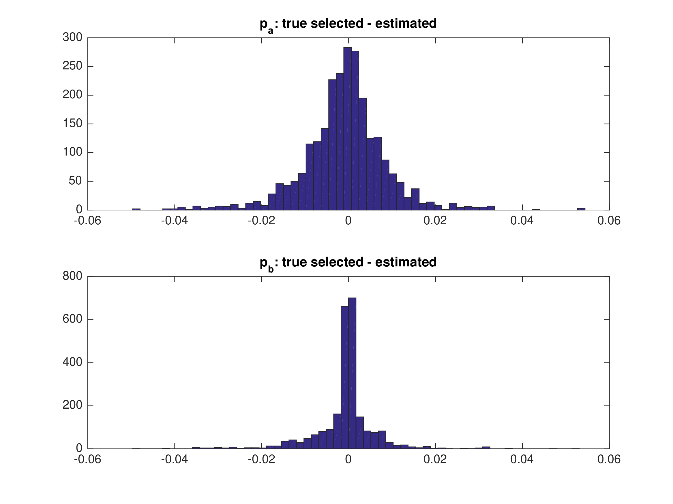
MPEC: Monte Carlo — Multiple Markets (\(M=2, T=625\))

Random equilibrium selection in different markets.

NFXP: Monte Carlo — Multiple Markets (\(M=25, T=50\))

Starting values \(\alpha_{0}=\alpha\), \(\beta_{0}=\beta\). Random equilibrium selection across markets.

MPEC: Monte Carlo — Multiple Markets (\(M=25, T=50\))

Starting values \(\alpha_{0}=\alpha\), \(\beta_{0}=\beta\). Random equilibrium selection across markets.

MPEC: Monte Carlo — Multiple Markets (\(M=2, T=625\))

Random equilibrium selection in different markets.

Discussion: NFXP

• 2 parameters in the optimization problem.

• Can identify the equilibrium played in the data, \(p_{a}^{m,k*}\) and \(p_{b}^{m,k*}\)
  (but in models with observationally equivalent equilibria this may not be possible).

• Needs to find all equilibria in each market (very hard in more complex problems).

• Good full-solution methods required.

Discussion: MPEC

• \(2+2M\) parameters in the optimization problem.

• Does not always converge to the equilibrium played in the data, although NFXP may indicate \(p_{a}^{m,k*}\) and \(p_{b}^{m,k*}\) are identifiable.

• Local minima with many markets.

• Disclaimer: quick and dirty MPEC implementation; prefer AMPL/Knitro.

2-Step CCP-based methods

Recall the FIML constrained formulation:

\[ \max_{\alpha,\beta,\, p^{m}_{a}, p^{m}_{b}} \ \log \mathcal{L}(p^{m}_{a}, p^{m}_{b};X) \]

subject to

\[ p^{m}_{a}= \Psi_{a}(p^{m}_{b},x^{m}_{a};\alpha,\beta),\qquad p^{m}_{b}= \Psi_{b}(p^{m}_{a},x^{m}_{b};\alpha,\beta), \]

\[ 0\le p^{m}_{a},p^{m}_{b}\le 1,\quad m=1,\dots,M. \]

• Denote the solution \((\alpha^{*},\beta^{*}, p^{*}_{a}, p^{*}_{b})\).

• Suppose \((p^{*}_{a}, p^{*}_{b})\) are known—how to recover \((\alpha^{*},\beta^{*})\)?

2-Step Methods: Recovering \((\alpha^{*},\beta^{*})\)

• Idea 1

  • Step 1: Estimate \(\hat{p}=(\hat{p}_{a},\hat{p}_{b})\) from the data.

  • Step 2: Solve the BNE equations for \((\alpha,\beta)\) given \((p^{*}_{a}, p^{*}_{b})\):

\[ \hat{p}_{a}= \Psi_{a}(\hat{p}_{b},x_{a};\alpha,\beta),\qquad \hat{p}_{b}= \Psi_{b}(\hat{p}_{a},x_{b};\alpha,\beta). \]

• Idea 2

  • Step 1: Estimate \(\hat{p}=(\hat{p}_{a},\hat{p}_{b})\) from the data.

  • Step 2: Choose \((\alpha,\beta)\) to

\[ \max_{\alpha,\beta}\ \log \mathcal{L}\!\big(\Psi_{a}(\hat{p}_{b},x_{a};\alpha,\beta),\ \Psi_{b}(\hat{p}_{a},x_{b};\alpha,\beta); X\big). \]

2-Step Methods: Potential Issues to Address

• How to estimate \(\hat{p}=(\hat{p}_{a},\hat{p}_{b})\)?

• Different methods yield different \(\hat{p}\).

• Frequency estimator:

\[ \hat{p}_{a}=\frac{1}{N}\sum_{i=1}^{N}\mathbf{1}\{d_{a}^{i}=1\},\qquad \hat{p}_{b}=\frac{1}{N}\sum_{i=1}^{N}\mathbf{1}\{d_{b}^{i}=1\}. \]

• If \((\hat{p}_{a},\hat{p}_{b})\ne (p^{*}_{a},p^{*}_{b})\) then \((\hat{\alpha},\hat{\beta})\ne (\alpha^{*},\beta^{*})\)

• For a given \((\hat{p}_{a},\hat{p}_{b})\), a solution to the BNE equations may not exist

Nested and 2-Step Pseudo Maximum Likelihood (NPL)

In 2-step methods:

• Step 1: Estimate \(\hat{p}=(\hat{p}_{a},\hat{p}_{b})\) from the data.

• Step 2: Solve

\[ \max_{\alpha,\beta,\, p_{a}, p_{b}}\ \log \mathcal{L}(p_{a}, p_{b};X) \]

• subject to

\[ p_{a}= \Psi_{a}(\hat{p}_{b},x_{a};\alpha,\beta),\qquad p_{b}= \Psi_{b}(\hat{p}_{a},x_{b};\alpha,\beta),\qquad 0\le p_{a},p_{b}\le 1. \]

• Equivalently:

  • Step 1: Estimate \(\hat{p}\).

  • Step 2: Solve

\[ \max_{\alpha,\beta}\ \log \mathcal{L}\!\big(\Psi_{a}(\hat{p}_{b},x_{a};\alpha,\beta),\ \Psi_{b}(\hat{p}_{a},x_{b};\alpha,\beta); X\big). \]

Least Squares Estimators

📖 Pesendorfer and Schmidt-Dengler [2008]

• Step 1: Estimate \(\hat{p}=(\hat{p}_{a},\hat{p}_{b})\) from the data.

• Step 2: Solve

\[ \min_{\alpha,\beta}\ \left\{ \big[\hat{p}_{a}-\Psi_{a}(\hat{p}_{b},x_{a};\alpha,\beta)\big]^{2} + \big[\hat{p}_{b}-\Psi_{b}(\hat{p}_{a},x_{b};\alpha,\beta)\big]^{2} \right\}. \]

For dynamic games, MPE conditions are \(p=\Psi(p,\theta)\).

• Step 1: Estimate \(\hat{p}\) from the data.

• Step 2: Solve

\[ \min_{\theta}\ [\hat{p}-\Psi(\hat{p};\theta)]' W [\hat{p}-\Psi(\hat{p};\theta)]. \]

Static Game Example: 2-Step PML (Eq 1)

Data generated from equilibrium 1

Static Game Example: 2-Step PML (Eq 2)

Data generated from equilibrium 2

Static Game Example: 2-Step PML (Eq 3)

Data generated from equilibrium 3

Nested Pseudo Likelihood (NPL):

📖 Aguirregabiria and Mira [2007]

NPL iterates on the 2-step method:

1. Step 1: Estimate \(\hat{p}^{0}=(\hat{p}^{0}_{a},\hat{p}^{0}_{b})\) from the data; set \(k=0\).

2. Step 2: Repeat

   1. Solve

\[ \alpha^{k+1},\beta^{k+1}=\arg\max_{\alpha,\beta}\ \log \mathcal{L}\!\big(\Psi_{a}(\hat{p}^{k}_{b},x_{a};\alpha,\beta),\ \Psi_{b}(\hat{p}^{k}_{a},x_{b};\alpha,\beta); X\big). \]

2. One best-reply iteration on \(\hat{p}^{k}\):

\[ \hat{p}_{a}^{k+1}= \Psi_{a}(\hat{p}_{b}^{k},x_{a};\alpha^{k+1},\beta^{k+1}),\qquad \hat{p}_{b}^{k+1}= \Psi_{b}(\hat{p}_{a}^{k},x_{b};\alpha^{k+1},\beta^{k+1}). \]

3. Let \(k\leftarrow k+1\)

Until convergence in \((\alpha^{k},\beta^{k})\) and \((\hat{p}^{k}_{a},\hat{p}^{k}_{b})\).

Monte Carlo Results: NPL with Eq 1

Equilibrium 1 — \(\hat{p}_{j}=\frac{1}{N}\sum_{i}\mathbf{1}(d_{j}=1)\)

Monte Carlo Results: NPL with Eq 2

Equilibrium 2 — \(\hat{p}_{j}=\frac{1}{N}\sum_{i}\mathbf{1}(d_{j}=1)\)

Monte Carlo Results: NPL with Eq 3

Equilibrium 3 — \(\hat{p}_{j}=\frac{1}{N}\sum_{i}\mathbf{1}(d_{j}=1)\)

Conclusions

• NFXP/MPEC implementations of MLE are statistically efficient but computationally daunting.

• Two-step estimators are computationally fast, but inefficient and biased in small samples.

• NPL (Aguirregabiria and Mira 2007) aims to bridge the gap, but may be unsuitable for games with multiple equilibria.

• Estimating even static games is an interesting yet challenging computational optimization problem:

  • Multiple equilibria can make the likelihood function discontinuous \(\rightarrow\) non-standard inference and computational complexity.

  • Multiple equilibria lead to indeterminacy and identification issues.

• All these problems are amplified in dynamic models.

Practical Task 7.3

• Find full Matlab implementation of Su(2014) static model

• Study the code to identify the parts that correspond to the lecture notes

• Identify where different estimators are implemented

• [otpional] Convert Matlab code to Python

Find the exercise code and materials in the exercises repo in the forlder 7_multiplicity/matlab_sgame

References and Additional Resources

• 📖 Su [2014] “Estimating discrete-choice games of incomplete information: Simple static examples”

• 📖 Egesdal et al. [2015] “Estimating dynamic discrete-choice games of incomplete information”

• Newton method with brackets for solving non-linear equations link