📖 Dynamic Entry Games#
⏱ | words
Code study task 6.1 Code study task 6.2 References
Dynamic games finally! 🥳#
Overall setup:
Several decision makers (players) make (discrete) choices over time
Maximize discounted expected utility/profit
Anticipate consequences of their current actions
Anticipate actions by other players in current and future periods
Solution of the model = equilibrium strategies that constitute mutual best responses
Key components of dynamic games:
State space of the model
Classification as in single agent models
In addition: what players know about different state variables?
Privite information and common knowledge
Action space of the players as in single agent models
Classification as in single agent models
Policy function = strategy
Strategy profile = collection of strategies of all players
Pure - mixed - behavioral strategies
Payoff function
As utility in single agent models
Describes preferences
Depends on all state variables and actions of all the players \(\implies\) strategic interaction
Transition rules for the state variables
Typically Markovian
Depend on actions of all players
Describe (common?) beliefs about the evolution of the future X
Markov Perfect Equilibrium#
is the most widely used concept of equilibrium in empirical dynamic games in IO and other fields, seminar works by Eric Maskin and Jean Tirole
📚 Maskin and Tirole [1988], Maskin and Tirole [1988], Maskin and Tirole [2001]
Loose definition
Markov Perfect Equilibrium (MPE) is given by a strategy profile (and associated value functions) such that all players are playing strategies that maximize their expected discounted utility/profit and these strategies constitute mutual best responses to all other players’ play.
Bellman equations hold for all players
Strategies correspond to the \(\arg\max\) actions in the Bellman equations
What about solving for MPE?#
Existence?
Uniqueness?
Main challenge: contraction mapping arguments do not apply in case of multiple players!
Iterative successive approximations (value function iterations) [Ericson and Pakes, 1995, Pakes and McGuire, 1994]
Solving players’ problems in order
Algebraic approach [Judd et al., 2012]
Based on recognizing the algebraic structure of equations that define MPE
Homotopy based methods [Borkovsky et al., 2008]
Follow a path from the area of easy solution to more complex solutions
Specific for subclasses of games
Supermodular games [Jia, 2008]
Directional games \(\rightarrow\) Recursive Lexicographical Search [Iskhakov et al., 2016]
Solving for all MPE in case of multiplicity is generally impossible!
What difficulties do you expect in estimation?
What about estimation?#
All the methods we have seen so far apply! Plus some more:
CCP 2-step methods [Bajari et al., 2007, Pakes et al., 2007, Pesendorfer and Schmidt-Dengler, 2008]
avoids full solution, but is inefficient and suffer from small sample bias
Nested Pseudo-Likelihood (NPL) [Aguirregabiria and Mira, 2007, Pesendorfer and Schmidt-Dengler, 2010]
middle ground between CCP and MLE
iterative method
convergence not guaranteed
Efficient Pseudo-Likelihood (EPL) [Dearing and Blevins, 2025]
Newton iteration ideas for NPL
more stable and efficient
more favorable statistical properties
convergence not guaranteed
Mathematical Programming with Equilibrium Constraints (MPEC) [Su and Judd, 2012]
probably most suitable MLE for the dynamic games
avoids repeated solution of all MPE, but suffer from serious issues with local minima
Nested Maximum Likelihood Estimation = Nested RLS in directional dynamic games [Iskhakov et al., n.d.]
needs to repeatedly solve for all MPE for every evaluation of the likelihood function
is it even possible?
Aguirregabiria and Mira (2007)#
📖 Aguirregabiria and Mira [2007] “Sequential Estimation of Dynamic Discrete Games”
📖 Egesdal et al. [2015] “Estimating dynamic discrete-choice games of incomplete information”
Entry/Exit Games: An Illustrative Example#
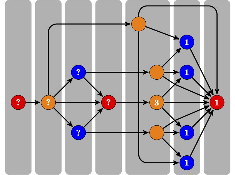
Five firms: \(i = 1,\dots,N=5\).
Firm \(i\)’s decision in period \(t\):
\[ a_i^t = 0:\ \text{exit (inactive)};\quad a_i^t = 1:\ \text{enter (active).} \]Simultaneous decisions conditional on observing the market size, all firms’ decisions in the last period, and private shocks.
Time |
Market Size |
Firm 1 |
Firm 2 |
Firm 3 |
Firm 4 |
Firm 5 |
|---|---|---|---|---|---|---|
0 |
2 |
0 |
0 |
0 |
0 |
0 |
1 |
3 |
0 |
1 |
0 |
0 |
1 |
2 |
4 |
0 |
1 |
0 |
1 |
1 |
3 |
5 |
0 |
1 |
0 |
0 |
1 |
4 |
5 |
1 |
1 |
0 |
0 |
0 |
5 |
5 |
1 |
1 |
0 |
0 |
1 |
6 |
6 |
1 |
1 |
1 |
1 |
1 |
⋮ |
⋮ |
⋮ |
⋮ |
⋮ |
⋮ |
⋮ |
General setup and notation#
Discrete-time infinite horizon: \(t = 1, 2, \dots, \infty\).
\(N\) players: \(i \in \mathcal{I} = \{1,\dots,N\}\).
Market size \(s^t \in \mathcal{S} = \{s_1,\dots,s_L\}\).
Market size is observed by all players.
Exogenous and stationary transition: \(f_{\mathcal{S}}(s_{t+1}\mid s_t)\).
At the beginning of period \(t\), player \(i\) observes \((x^t, \varepsilon_i^t)\).
\(x_t\): a vector of common-knowledge state variables.
\(\varepsilon_i^t\): private shocks.
Players simultaneously choose whether to be active in the market in that period.
\(a_i^t \in \mathcal{A} = \{0,1\}\): player \(i\)’s action in period \(t\).
\(a^t = (a_1^t,\dots,a_N^t)\): all players’ actions.
\(a_{-i}^t = (a_1^t,\dots,a_{i-1}^t, a_{i+1}^t,\dots,a_N^t)\): actions of all players other than \(i\).
State Variables#
Common-knowledge state variables: \(\mathbf{x}_t = (s_t, \mathbf{a}^{t-1})\).
Private shocks: \(\varepsilon_i^t = \{\varepsilon_i^t(a_i^t)\}_{a_i^t \in \mathcal{A}}\).
\(\varepsilon_i^t(a_i^t)\) is i.i.d. type-I extreme value across actions, players, and time.
Opposing players know only its density \(g(\varepsilon_i^t)\).
Conditional independence assumption on state transition:
\[ p\!\left[\mathbf{x}^{t+1}=(s',\mathbf{a}'),\, \varepsilon_i^{t+1}\mid \mathbf{x}^t=(s,\tilde{\mathbf{a}}),\, \varepsilon_i^t,\, \mathbf{a}^t\right] = f_{\mathcal{S}}(s'\mid s)\,\mathbf{1}\{\mathbf{a}'=\mathbf{a}^t\}\, g(\varepsilon_i^{t+1}). \]
Player \(i\)’s Utility Maximization Problem#
\(\boldsymbol{\theta}\): vector of structural parameters.
\(\beta \in (0,1)\): discount factor.
Per-period payoff:
\[ \tilde{\Pi}_i(a_i^t,\mathbf{a}_{-i}^t,\mathbf{x}^t,\boldsymbol{\varepsilon}_i^t;\boldsymbol{\theta}) = \Pi_i(a_i^t,\mathbf{a}_{-i}^t,\mathbf{x}^t;\boldsymbol{\theta}) + \boldsymbol{\varepsilon}_i^t(a_i^t). \]Common-knowledge component:
\[\begin{split} \Pi_i(a_i^t,\mathbf{a}_{-i}^t,\mathbf{x}^t;\boldsymbol{\theta}) = \begin{cases} \theta^{RS}s^t - \theta^{RN}\log\!\Big\{1+\sum_{j\neq i} a_j^t\Big\} - \theta^{FC} - \theta^{EC}(1-a_i^{t-1}), & a_i^t=1,\\[4pt] 0, & a_i^t=0. \end{cases} \end{split}\]Player \(i\)’s problem:
\[ \max_{\{a_i^t,a_i^{t+1},\dots\}} \mathbb{E}\!\left[\sum_{\tau=t}^{\infty} \beta^{\tau -t} \tilde{\Pi}_i(a_i^\tau,\mathbf{a}_{-i}^\tau,\mathbf{x}^\tau,\boldsymbol{\varepsilon}_i^\tau;\boldsymbol{\theta}) \,\middle|\, (\mathbf{x}^t,\boldsymbol{\varepsilon}_i^t)\right]. \]
Equilibrium (MPE)#
Characterization in terms of observed states \(\mathbf{x}\).
\(P_i(a_i\mid \mathbf{x})\): conditional choice probability for player \(i\) at state \(\mathbf{x}\).
\(V_i(\mathbf{x})\): integrated value function for player \(i\) at state \(\mathbf{x}\).
Define \(\mathbf{P}=\{P_i(a_i\mid \mathbf{x})\}_{i\in\mathcal{I}, a_i\in\mathcal{A}, \mathbf{x}\in\mathcal{X}}\) and \(\mathbf{V}=\{V_i(\mathbf{x})\}_{i\in\mathcal{I}, \mathbf{x}\in\mathcal{X}}\).
System I: Bellman Optimality#
For all \(i\in\mathcal{I}\), \(\mathbf{x}\in\mathcal{X}\):
\[ V_i(\mathbf{x})=\sum_{a_i\in\mathcal{A}} P_i(a_i\mid \mathbf{x}) \big[\pi_i(a_i\mid \mathbf{x},\boldsymbol{\theta}) + e_i^{\mathbf{P}}(a_i\mid \mathbf{x})\big] + \beta \sum_{\mathbf{x}'\in\mathcal{X}} V_i(\mathbf{x}')\, f_{\mathcal{X}}^{\mathbf{P}}(\mathbf{x}'\mid \mathbf{x}). \]\(\pi_i(a_i\mid \mathbf{x},\boldsymbol{\theta})\): expected payoff from choosing \(a_i\) at state \(\mathbf{x}\) given \(\{P_j(a_j\mid \mathbf{x})\}\),
\[ \pi_i(a_i\mid \mathbf{x},\boldsymbol{\theta}) = \sum_{a_{-i}\in\mathcal{A}^{N-1}} \left\{ \left[\prod_{a_j\in \mathbf{a}_{-i}} P_j(a_j\mid \mathbf{x}) \right] \Pi_i(a_i,\mathbf{a}_{-i},\mathbf{x};\boldsymbol{\theta}) \right\}. \]State transition for \(\mathbf{x}\) given \(\mathbf{P}\):
\[ f_{\mathcal{X}}^{\mathbf{P}}(\mathbf{x}'=(s',\mathbf{a}')\mid \mathbf{x}=(s,\tilde{\mathbf{a}})) = \Big[\prod_{j=1}^N P_j(a'_j\mid \mathbf{x})\Big]\, f_{\mathcal{S}}(s'\mid s). \]
Which type of the value function do we have here?
With i.i.d. extreme value shocks (scale \(\sigma\)), the conditional expectation:
\[ e_i^{\mathbf{P}}(a_i\mid \mathbf{x}) = \text{Euler-Mascheroni constant} - \sigma \log P_i(a_i\mid \mathbf{x}). \]
System II: Bayes–Nash Equilibrium Conditions#
For all \(i\in\mathcal{I}\), \(j\in\mathcal{A}\), \(\mathbf{x}\in\mathcal{X}\):
\[ P_i(a_i=j\mid \mathbf{x})= \frac{\exp\big[v_i(a_i=j\mid \mathbf{x})\big]} {\sum_{k\in\mathcal{A}} \exp\big[v_i(a_i=k\mid \mathbf{x})\big]}. \]Choice-specific value functions:
\[ v_i(a_i=j\mid \mathbf{x}) = \pi_i(a_i\mid \mathbf{x},\boldsymbol{\theta}) + \beta \sum_{\mathbf{x}'\in\mathcal{X}} V_i(\mathbf{x}')\, f_i^{\mathbf{P}}(\mathbf{x}'\mid \mathbf{x}, a_i). \]Conditional transition:
\[ f_i^{\mathbf{P}}(\mathbf{x}'=(s',\mathbf{a}')\mid \mathbf{x}=(s,\tilde{\mathbf{a}}), a_i) = f_{\mathcal{S}}(s'\mid s)\,\mathbf{1}\{a'_i=a_i\} \prod_{j\in \mathcal{I}\setminus\{i\}} P_j(a'_j\mid \mathbf{x}). \]
Markov Perfect Equilibrium (Compact Form)#
Bellman:
\[ V_i(\mathbf{x})=\sum_{a_i\in\mathcal{A}} P_i(a_i\mid \mathbf{x}) \big[\pi_i(a_i\mid \mathbf{x},\boldsymbol{\theta}) + e_i^{\mathbf{P}}(a_i\mid \mathbf{x})\big] + \beta \sum_{\mathbf{x}'\in\mathcal{X}} V_i(\mathbf{x}')\, f_{\mathcal{X}}^{\mathbf{P}}(\mathbf{x}'\mid \mathbf{x}). \]Bayes–Nash:
\[ P_i(a_i=j\mid \mathbf{x})= \frac{\exp\big[v_i(a_i=j\mid \mathbf{x})\big]} {\sum_{k\in\mathcal{A}} \exp\big[v_i(a_i=k\mid \mathbf{x})\big]}. \]Compact notation:
\[ \mathbf{V}=\Psi^{\mathbf{V}}(\mathbf{V},\mathbf{P},\boldsymbol{\theta}),\qquad \mathbf{P}=\Psi^{\mathbf{P}}(\mathbf{V},\mathbf{P},\boldsymbol{\theta}). \]Set of all MPE:
\[ SOL(\Psi,\boldsymbol{\theta}) = \big\{(\mathbf{P},\mathbf{V}) \,\big|\, \mathbf{V}=\Psi^{\mathbf{V}}(\mathbf{V},\mathbf{P},\boldsymbol{\theta}),\ \mathbf{P}=\Psi^{\mathbf{P}}(\mathbf{V},\mathbf{P},\boldsymbol{\theta}) \big\}. \]
Econometric model and data generating process#
\(\boldsymbol{\theta}_0\): true structural parameters in the population.
\((\mathbf{V}^0,\mathbf{P}^0)\): a Markov Perfect Equilibrium at \(\boldsymbol{\theta}_0\).
Assumptions:
If multiple MPE exist, only one equilibrium is played in the data.
Stationarity: the same equilibrium is played outside of the sample periods
Independence across markets
Standard identification assumption
(See Assumption 5 in AM 2007 for details.)
Data: \(\mathbf{Z}=\{\bar{\mathbf{a}}^{mt}, \bar{\mathbf{x}}^{mt}\}_{m\in\mathcal{M}, t\in\mathcal{T}}\).
Observations from \(M\) independent markets over \(T\) periods.
In each market \(m\) and time \(t\):
Common-knowledge state variables \(\bar{\mathbf{x}}^{mt}\).
Players’ actions \(\bar{\mathbf{a}}^{mt}=(\bar{a}_1^{mt},\dots,\bar{a}_N^{mt})\).
Estimation#
Maximum-Likelihood Estimation#
For a given \(\boldsymbol{\theta}\), let \((\mathbf{P}^\ell(\boldsymbol{\theta}), \mathbf{V}^\ell(\boldsymbol{\theta})) \in SOL(\Psi,\boldsymbol{\theta})\) denote the \(\ell\)-th equilibrium.
Given data \(\mathbf{Z}\), the log-likelihood is:
\[ \mathcal{L}(\mathbf{Z},\boldsymbol{\theta}) = \max_{(\mathbf{P}^\ell(\boldsymbol{\theta}),\mathbf{V}^\ell(\boldsymbol{\theta}))\in SOL(\Psi,\boldsymbol{\theta})} \frac{1}{M}\sum_{i=1}^N \sum_{m=1}^M \sum_{t=1}^T \log P_i^{\ell}(\bar{a}_i^{mt}\mid \bar{\mathbf{x}}^{mt}; \boldsymbol{\theta}). \]ML estimator:
\[ \boldsymbol{\theta}^{ML}=\arg\max_{\boldsymbol{\theta}} \mathcal{L}(\mathbf{Z},\boldsymbol{\theta}). \]
Structural Estimation via Constrained Optimization (MPEC)#
Given \(\mathbf{Z}\), define the (augmented) log-likelihood:
\[ \mathcal{L}(\mathbf{Z},\mathbf{P}) = \frac{1}{M}\sum_{i=1}^N \sum_{m=1}^M \sum_{t=1}^T \log P_i(\bar{a}_i^{mt}\mid \bar{\mathbf{x}}^{mt}; \boldsymbol{\theta}). \]Constrained ML formulation:
\[\begin{split} \begin{aligned} \max_{(\boldsymbol{\theta},\mathbf{P},\mathbf{V})}\quad & \mathcal{L}(\mathbf{Z},\mathbf{P})\\ \text{s.t.}\quad & \mathbf{V}=\Psi^{\mathbf{V}}(\mathbf{V},\mathbf{P},\boldsymbol{\theta}),\\ & \mathbf{P}=\Psi^{\mathbf{P}}(\mathbf{V},\mathbf{P},\boldsymbol{\theta}). \end{aligned} \end{split}\]Theorem: Constrained and unconstrained problems have the same solutions.
Solving All Equilibria in ML Estimation?#
Motivation for MPEC: It is often stated that under the constrained approach, one need not solve for all equilibria at each parameter guess.
Constraints are enforced (and an equilibrium solved) only at a solution, not at every iteration.
The optimizer needs only equilibria/parameters that are local solutions satisfying FOCs.
These features eliminate many equilibria/parameters that do not need to be solved.
Are you convinced? What could go wrong?
Two-Step Methods: Intuition#
Recall the constrained ML problem above. Denote the solution by \((\boldsymbol{\theta}^*,\mathbf{P}^*,\mathbf{V}^*)\).
Suppose \(\mathbf{P}^*\) is known—how do we recover \(\boldsymbol{\theta}^*\) (and \(\mathbf{V}^*\))?
Two-Step Pseudo Maximum-Likelihood (2S-PML)#
Step 1: Nonparametrically estimate the CCPs \(\hat{\mathbf{P}}\) from data \(\mathbf{Z}\).
Step 2: Solve
\[\begin{split} \begin{aligned} \max_{(\boldsymbol{\theta},\mathbf{P},\mathbf{V})}\quad & \mathcal{L}(\mathbf{Z},\mathbf{P})\\ \text{s.t.}\quad & \mathbf{V}=\Psi^{\mathbf{V}}(\mathbf{V},\hat{\mathbf{P}},\boldsymbol{\theta}),\\ & \mathbf{P}=\Psi^{\mathbf{P}}(\mathbf{V},\hat{\mathbf{P}},\boldsymbol{\theta}), \end{aligned} \end{split}\]or equivalently,
\[\begin{split} \begin{aligned} \max_{(\boldsymbol{\theta},\mathbf{V})}\quad & \mathcal{L}\!\big(\mathbf{Z},\,\Psi^{\mathbf{P}}(\mathbf{V},\hat{\mathbf{P}},\boldsymbol{\theta})\big)\\ \text{s.t.}\quad & \mathbf{V}=\Psi^{\mathbf{V}}(\mathbf{V},\hat{\mathbf{P}},\boldsymbol{\theta}). \end{aligned} \end{split}\]
Reformulation in Step 2#
Bellman (stacked) notation. Define
\(\mathbf{V}_i=[V_i(x)]_{\mathbf{x}\in\mathcal{X}}\),
\(\hat{\mathbf{P}}_i(a_i)=[\hat{P}_i(a_i)(x)]_{\mathbf{x}\in\mathcal{X}}\),
\(\mathbf{e}_i^{\mathbf{P}}(a_i)=[e_i^{\mathbf{P}}(a_i\mid \mathbf{x})]_{\mathbf{x}\in\mathcal{X}}\),
\(\boldsymbol{\pi}_i(a_i,\boldsymbol{\theta})=[\pi_i(a_i\mid \mathbf{x},\boldsymbol{\theta})]_{\mathbf{x}\in\mathcal{X}}\),
\(\mathbf{F}_{\mathcal{X}}^{\hat{\mathbf{P}}}=[f_{\mathcal{X}}^{\mathbf{P}}(\mathbf{x}'\mid \mathbf{x})]_{\mathbf{x},\mathbf{x}'\in\mathcal{X}}\).
Then
\[ \big[\mathbf{I}-\beta \mathbf{F}_{\mathcal{X}}^{\hat{\mathbf{P}}}\big]\mathbf{V}_i = \sum_{a_i\in\mathcal{A}} \big[\hat{\mathbf{P}}_i(a_i)\times \boldsymbol{\pi}_i(a_i,\boldsymbol{\theta})\big] + \sum_{a_i\in\mathcal{A}} \big[\hat{\mathbf{P}}_i(a_i)\times \mathbf{e}_i^{\mathbf{P}}(a_i)\big], \]hence
\[ \mathbf{V}_i = \big[\mathbf{I}-\beta \mathbf{F}_{\mathcal{X}}^{\hat{\mathbf{P}}}\big]^{-1} \left\{ \sum_{a_i\in\mathcal{A}} \big[\hat{\mathbf{P}}_i(a_i)\times \boldsymbol{\pi}_i(a_i,\boldsymbol{\theta})\big] + \sum_{a_i\in\mathcal{A}} \big[\hat{\mathbf{P}}_i(a_i)\times \mathbf{e}_i^{\mathbf{P}}(a_i)\big] \right\}. \]Compactly, \(\mathbf{V}=\Gamma(\boldsymbol{\theta},\hat{\mathbf{P}})\).
Eliminating \(\mathbf{V}\), Step 2 becomes:
\[ \max_{\boldsymbol{\theta}} \ \mathcal{L}\!\Big(\mathbf{Z}, \Psi^{\mathbf{P}}(\Gamma(\boldsymbol{\theta},\hat{\mathbf{P}}),\hat{\mathbf{P}},\boldsymbol{\theta})\Big). \]Define the 2S-PML estimator:
\[ \boldsymbol{\theta}^{2\text{S-PML}} = \arg\max_{\boldsymbol{\theta}} \mathcal{L}\!\Big(\mathbf{Z}, \Psi^{\mathbf{P}}(\Gamma(\boldsymbol{\theta},\hat{\mathbf{P}}),\hat{\mathbf{P}},\boldsymbol{\theta})\Big). \]
NPL Estimator#
2S-PML can have large finite-sample biases.
To reduce bias, Aguirregabiria and Mira (2007) propose NPL.
An NPL fixed point \((\tilde{\boldsymbol{\theta}},\tilde{\mathbf{P}})\) satisfies
\[ \tilde{\boldsymbol{\theta}} = \arg\max_{\boldsymbol{\theta}} \mathcal{L}\!\Big(\mathbf{Z},\Psi^{\mathbf{P}}(\Gamma(\boldsymbol{\theta},\tilde{\mathbf{P}}),\tilde{\mathbf{P}},\boldsymbol{\theta})\Big), \qquad \tilde{\mathbf{P}}=\Psi^{\mathbf{P}}(\Gamma(\boldsymbol{\theta},\tilde{\mathbf{P}}),\tilde{\mathbf{P}},\boldsymbol{\theta}). \]Algorithm (for \(1\le K\le \bar{K}\)):
Step 1: Given \(\tilde{\mathbf{P}}_{K-1}\), solve
\(\tilde{\boldsymbol{\theta}}_{K} = \arg\max_{\boldsymbol{\theta}} \mathcal{L}\!\big(\mathbf{Z},\Psi^{\mathbf{P}}(\Gamma(\boldsymbol{\theta},\tilde{\mathbf{P}}_{K-1}),\tilde{\mathbf{P}}_{K-1},\boldsymbol{\theta})\big)\).Step 2: Given \(\tilde{\boldsymbol{\theta}}_{K}\), update
\(\tilde{\mathbf{P}}_{K} = \Psi^{\mathbf{P}}(\Gamma(\boldsymbol{\theta}_{K},\tilde{\mathbf{P}}_{K-1}),\tilde{\mathbf{P}}_{K-1},\boldsymbol{\theta}_{K})\).
Empirical Application#
📖 Aguirregabiria and Mira [2007] “Sequential Estimation of Dynamic Discrete Games”
Chilean firm entry example#
Discrete-time infinite horizon: \(t = 1,2,\dots,\infty\).
\(N=5\) players: \(i\in\mathcal{I}=\{1,\dots,5\}\).
Market size \(s^t \in \mathcal{S}=\{1,\dots,5\}\).
Total number of grid points in the state space:
\[ |\mathcal{X}| = |\mathcal{S}| \times |\mathcal{A}|^N = 5 \times 2^5 = 160. \]Discount factor \(\beta=0.95\); type I EV scale \(\sigma=1\).
Common-knowledge per-period payoff:
\[\begin{split} \Pi_i(a_i^t,\mathbf{a}_{-i}^t,\mathbf{x}^t;\boldsymbol{\theta}) = \begin{cases} \theta^{RS}s^t - \theta^{RN}\log\!\Big\{1+\sum_{j\neq i} a_j^t\Big\} - \theta^{FC} - \theta^{EC}(1-a_i^{t-1}) +\omega_m, & a_i^t=1,\\[4pt] 0, & a_i^t=0. \end{cases} \end{split}\]\(\omega_m\): market-specific effect (unobserved heterogeneity, discretized)
Structural parameters \(\boldsymbol{\theta}=(\theta^{RS},\theta^{RN},\boldsymbol{\theta}^{FC},\theta^{EC})\) with \(\boldsymbol{\theta}^{FC}=\{\theta_i^{FC}\}_{i=1}^N\)
Focus on symmetric MPE equilibria
Descriptives#
The data come from a census of Chilean firms created for tax purposes by the Chilean Servicio de Impuestos Internos (Internal Revenue Service)
annual frequency and covers the years 1994–1999
data set at the firm level are
(i) firm identification number,
(ii) firm industry at the five digit level,
(iii) annual sales, discretized in 12 cells, and
(iv) the comuna (i.e., county) where the firm is located
authors combine these data with annual information on population at the level of comunas for every year between 1990 and 2003
five retail industries
comunas as local markets (with exclusion of large cities to avoid inter-market interactions)
separate model for each industry
measure of market size \(s_mt\) is the population in comuna \(m\) at year \(t\)
dynamics by AR(1) evolution in logs
discretized
transition probability matrix estimated from data
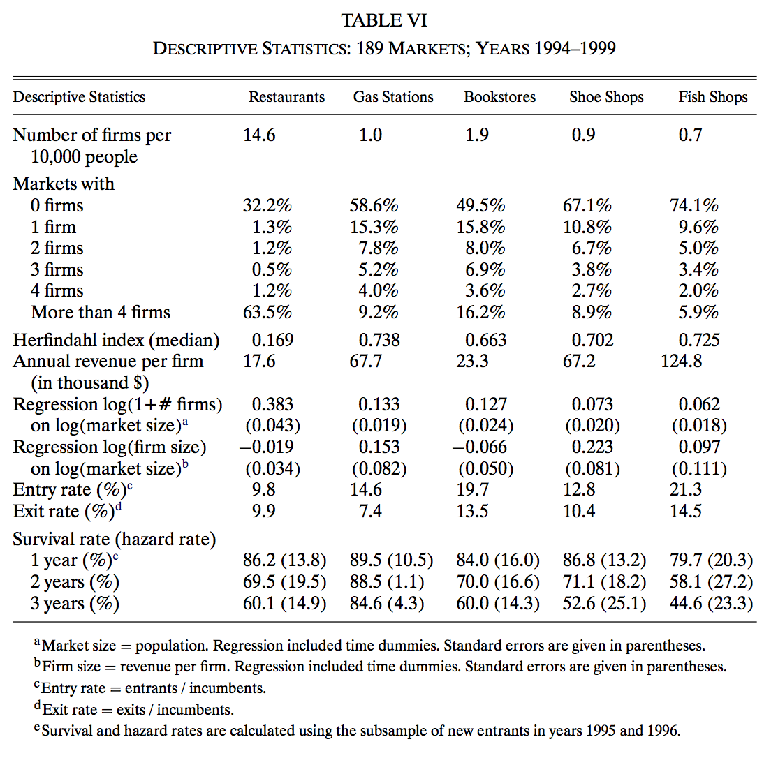
Some observations:
Why so many restaurants and so few gas stations and bookstores?
Market concentration is smaller in the restaurant industry.
Turnover rates are very high across retail industries.
Survival is more likely in gas stations than in other industries.
What explains these facts?
Economies of scale (smaller fixed cost for restaurants?)
Sunken entry costs (smaller for restaurants?)
Strategic interactions (is product differentiation possible for gas stations?)
Structural Estimates: Aguirregabiria and Mira (2007)#
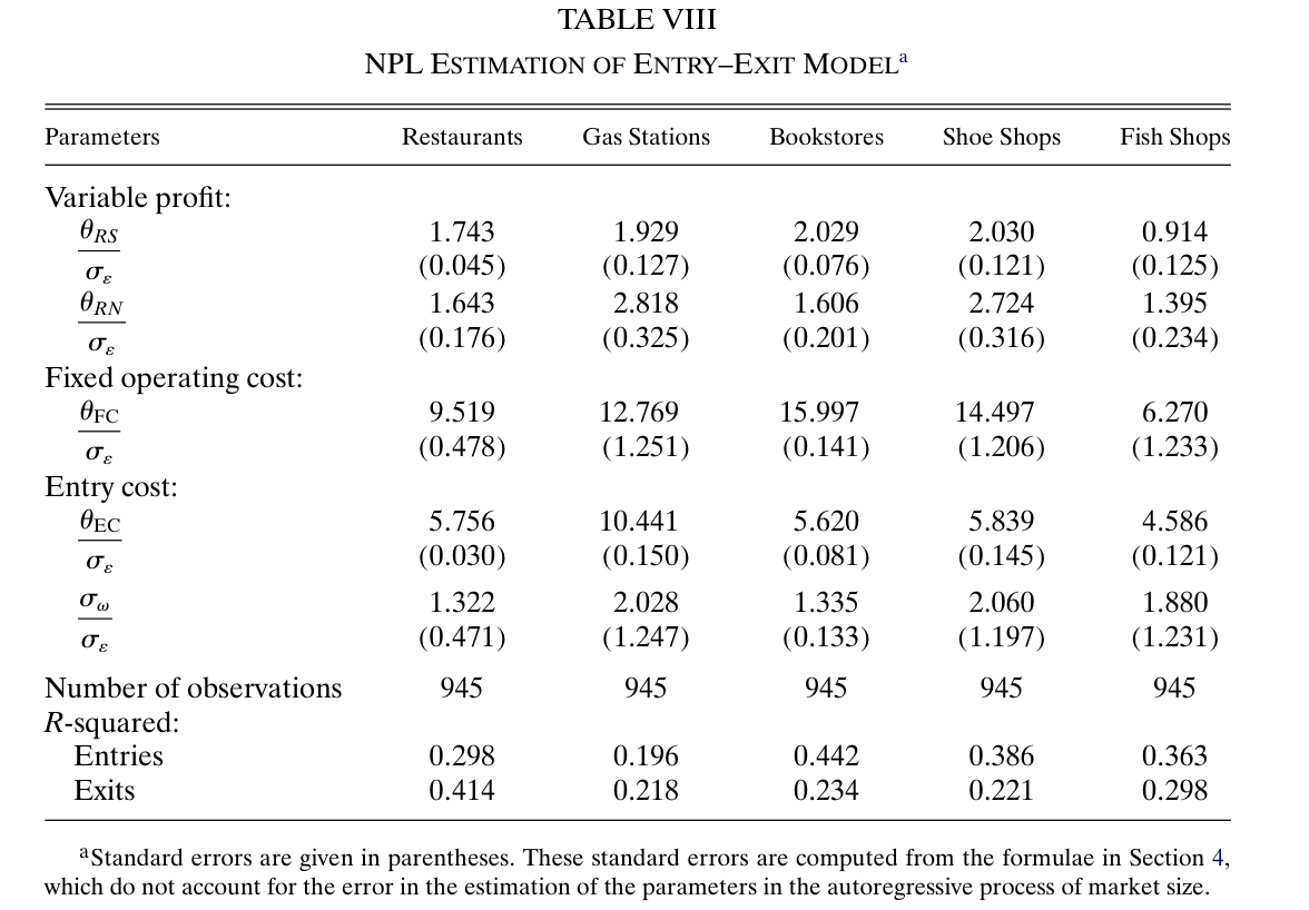
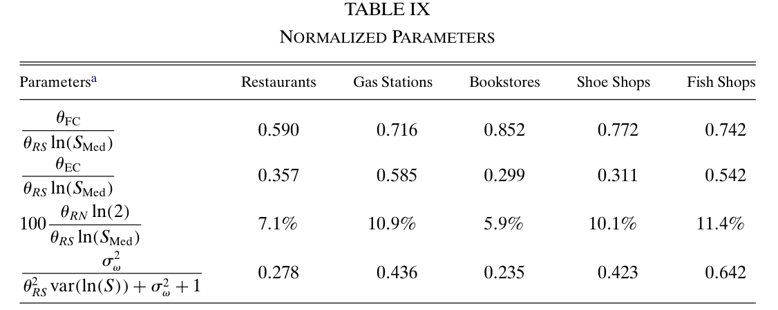
The normalized coefficients allow for cross-industry comparisons:
\(\theta_{FC}/(\theta_{RS}\ln S_{\text{med}})\): ratio of fixed operating costs to a monopolist’s variable profits in a median-size market.
\(\theta_{EC}/(\theta_{RS}\ln S_{\text{med}})\): ratio of sunk entry costs to a monopolist’s variable profits in a median-size market.
\(\theta_{RN}\ln(2)/(\theta_{RS}\ln S_{\text{med}})\): percent reduction in variable profits per firm from monopoly to duopoly in the median market.
\(\sigma_w^2/(\theta_{RS}^2\operatorname{var}(\ln S)+\sigma_w^2+1)\): percent of cross-market variability in monopoly profits explained by the unobserved market type.
Key takeaways from the estimates:
Fixed operating costs are a very important component of total profits.
Sunk entry costs are statistically significant in all five industries.
Gas stations have the largest sunk costs.
Strategic interaction parameter is statistically significant across industries.
Summary of Findings (AM 2007)#
Economies of scale are smaller in restaurants, explaining the large number of restaurants.
Strategic interactions are particularly small among restaurants and bookstores, possibly due to greater product differentiation—also contributing to many restaurants.
Economies of scale seem important in bookstores; nevertheless, bookstores outnumber gas stations and shoe shops due to weaker negative strategic interactions.
Sunk entry costs are significant across industries but smaller than annual fixed operating costs.
Gas stations have the largest sunk costs; this helps explain their lower turnover, though not necessarily fewer firms.
Monte Carlo experiments to compare estimation methods#
📖 Egesdal et al. [2015] “Estimating dynamic discrete-choice games of incomplete information”
Experiment 1#
Market size transition matrix \(f_{\mathcal{S}}(s^{t+1}\mid s^t)\):
\[\begin{split} \begin{pmatrix} 0.8 & 0.2 & 0 & \cdots & 0 & 0 \\ 0.2 & 0.6 & 0.2 & \cdots & 0 & 0 \\ \vdots & \vdots & \ddots & \ddots & \vdots & \vdots \\ 0 & 0 & \cdots & 0.2 & 0.6 & 0.2 \\ 0 & 0 & \cdots & 0 & 0.2 & 0.8 \end{pmatrix} \end{split}\]Market size: \(|\mathcal{S}|=5\) with \(\mathcal{S}=\{1,2,\dots,5\}\).
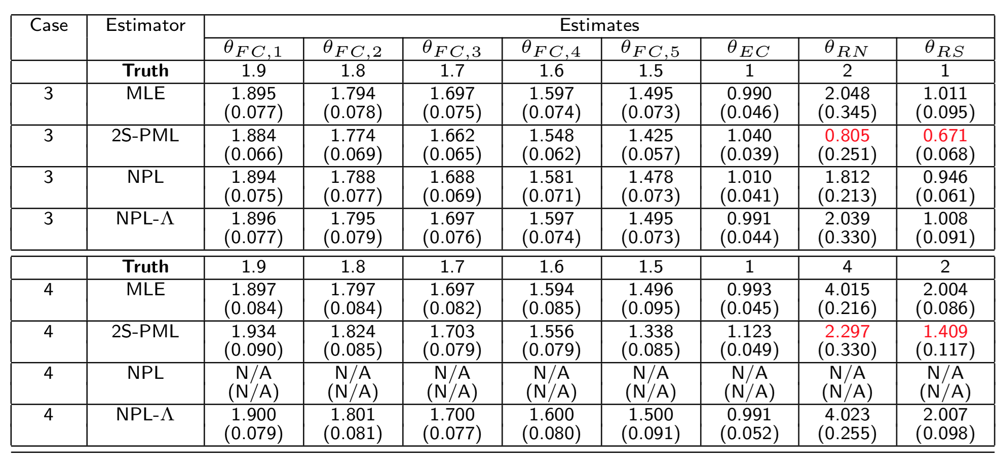
True parameters: \(\boldsymbol{\theta}^{FC}_0=(1.9,1.8,1.7,1.6,1.5)\) and \(\theta^{EC}_0=1\).
Two cases:
\((\theta^{RS},\theta^{RN})=(2,1)\),
\((\theta^{RS},\theta^{RN})=(4,2)\).
Experiment 2#
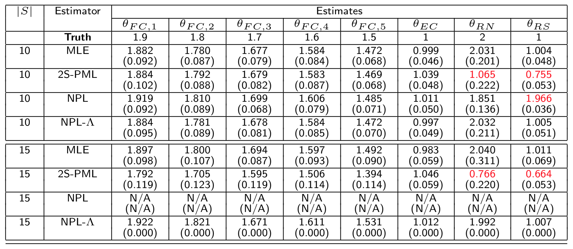
Two market-size grids:
\(|\mathcal{S}|=10\) with \(\mathcal{S}=\{1,\dots,10\}\)
→ ML solves a constrained problem with 4,800 constraints and 4,808 variables.\(|\mathcal{S}|=15\) with \(\mathcal{S}=\{1,\dots,15\}\)
→ ML solves a constrained problem with 7,200 constraints and 7,208 variables.
All other specifications as in Experiment 1.
Data Simulation and Implementation#
In each dataset: \(M=400\), \(T=10\).
For Cases 3–4 in Experiment 1:
100 datasets per case.
MPEC: 10 starting points per dataset.
For Cases 5–6 in Experiment 2:
50 datasets per case.
MPEC: 5 starting points per dataset.
For NPL and NPL–\(\Lambda\): \(\bar{K}=100\); for NPL–\(\Lambda\): \(\lambda=0.5\).
Monte Carlo Results#
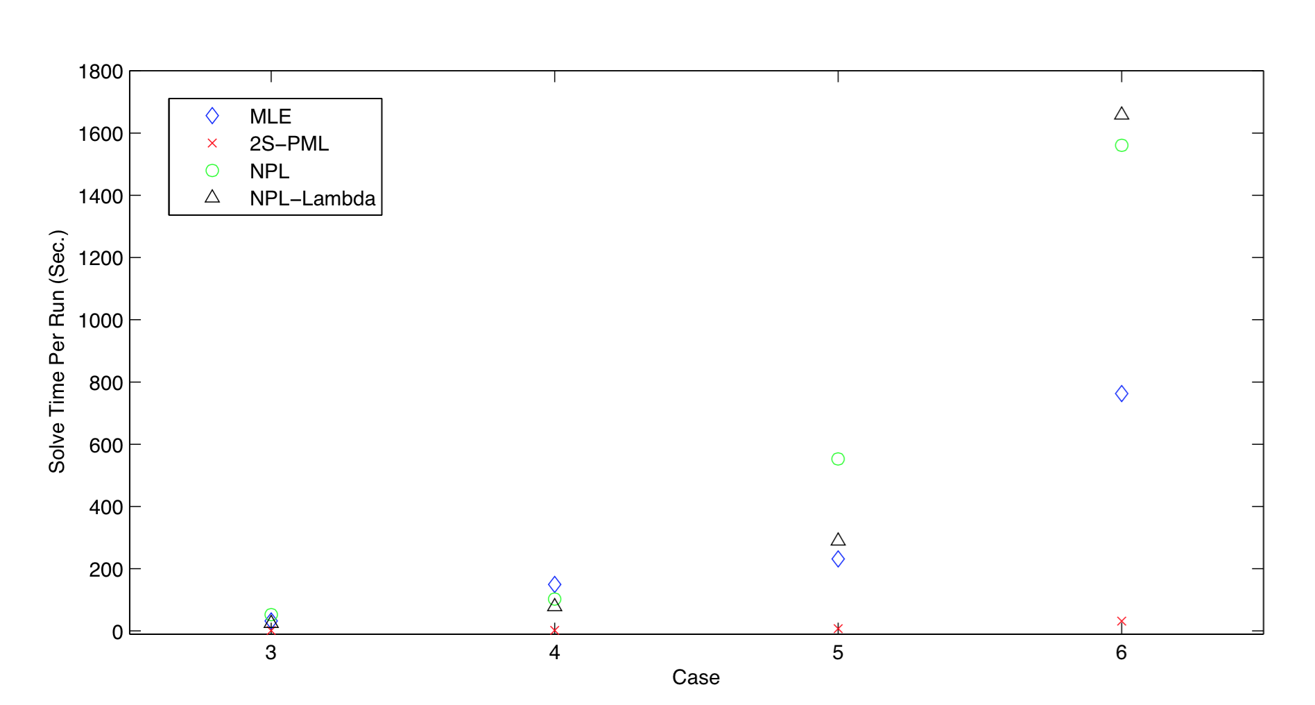
Average solve time per run
Estimates for Experiment 1
Estimates for Experiment 2
Findings#
Recursive methods are not always reliable computationally and should be used with caution
The 2S-PML estimator often exhibits large finite-sample biases
The constrained optimization approach is reliable and can estimate relevant dynamic game models such as AM (2007)
Open questions:
Improving constrained optimization performance for higher-dimensional state spaces
Is MPEC reliable under multiple equilibria?
We investigate this for a specific class of Dynamic Directional Games next week
Practical Task 6.1
Find the exercise code and materials in the exercises repo in the forlder 6_entry_npl/matlab/
Study and make sense of the code that implements the NPL estimator for the entry model in [Toivanen and Waterson, 2005]
Run the code under different specifications (requires Matlab)
Discuss the structure of the code: is it well modularized? Are independent tasks separated into functions, modules and classes?
Design a plan for translating the code to Python, thinking through the architecture of the code and how to make it efficient and modular
(There exercises are kindly provided by friends at the University of Copenhagen)
Practical Task 6.2
Study the presentation and replication of Aguirregabiria and Mira (2007) by Jason Blevins and Minhae Kim available at link to replication package .
Make sure you understand the structure of the code and its main functions
Comment on what is done well and not so well in the replication package in terms of code design.
Think through about a more efficient code architecture for translation to Python
[optional] Perform the translation part by part, running tests to make sure the translated code performs identical to the original code
References and Additional Resources
📖 Aguirregabiria and Mira [2007] “Sequential Estimation of Dynamic Discrete Games”
📖 Egesdal et al. [2015] “Estimating dynamic discrete-choice games of incomplete information”
📖 Aguirregabiria and Marcoux [2021] “Imposing equilibrium restrictions in the estimation of dynamic discrete games”
📖 Doraszelski and Escobar [2010] “A theory of regular Markov perfect equilibria in dynamic stochastic games: Genericity, stability, and purification”
📖 Toivanen and Waterson [2005] “Market Structure and Entry: Where’s the Beef?”
📖 Toivanen and Waterson [2000] “Empirical research on discrete choice game theory models of entry: An illustration”
“Nested Pseudo-Likelihood Estimation of Dynamic Discrete Choice Games: A Replication and Retrospective” by Jason Blevins and Minhae Kim link to replication package